The incidence of visual impairment and blindness caused by inherited retinal diseases (IRDs) is increasing because of prolonged life expectancy. A recent analysis shows approximately 5.5 million people worldwide have IRDs ^[1]. In recent years, several advancements have been made in the diagnosis and treatment of IRDs, including drug and gene therapies^[2-4]. Spectral-domain optical coherence tomography (SD-OCT) has played a crucial role in the diagnosis, progression surveillance, strategy exploration, and response assessment of treatment in patients with IRDs. However, in some cases, the recognition, interpretation, and comparison of minor changes in IRDs, as shown by OCT, could be difficult and time-consuming for retinal specialists.

Artificial intelligence technology is gaining popularity in retinal imaging owing to its enhanced processing power, massive data, and novel algorithms^[5]. Recently, automated image analysis has been successfully applied to detect changes in fundus and OCT images of multiple retinal diseases, such as diabetic retinopathy^[6], age-related macular degeneration (AMD)^[7], and glaucoma^[8]. These diseases are highly prevalent among populations and enable the acquisition of large volumes of training data for traditional machine learning (ML) approaches, including deep learning (DL).

In contrast, for rare diseases such as IRDs, acquiring a large volume of high-quality representative data from the patient cohort is challenging. Furthermore, the datasets require accompanying annotations generated by specialists, which is time-consuming. The scarcity of samples and laborious work hinder the application of image classification.

Therefore, researchers have imitated the fact that human beings can learn quickly and proposed few-shot learning (FSL). Unlike traditional networks, FSL aims to address the problem of data limitation when learning new tasks. This avoids the problems of parameter overfitting and a low model generalization performance. This shows greater adaptability to unknown conditions and provides a reliable solution for areas where samples are scarce.

This study aimed to design a diagnosis FSL model for the classification of OCT images in patients with IRDs when only a very limited number of samples can be collected.

A publicly available dataset of OCT images from the Cell dataset^[9] and BOE dataset^[10] was selected as the auxiliary dataset for training. The Cell dataset contains four classifications, including choroidal neovascularization (CNV), diabetic macular edema (DME), drusen, and normal, which total 109,309 samples with two image resolutions, 1,536 × 496 and 1,024 × 496 pixels. The BOE dataset has 3,231 samples, including dry AMD, DME, and normal, with three types of image resolution: 1,024 × 496, 768 × 496, and 512 × 496 pixels.

SD-OCT images of the target dataset were acquired using the Cirrus HD-OCT 5000 system (Carl Zeiss Meditec Inc., Dublin, USA) and the Heidelberg Spectralis system (Heidelberg Engineering, Heidelberg, Germany). An OCT scan containing the center of the fovea from each macular OCT was selected as the input data. Images from the Cirrus system were scanned at a length of 6 mm, and the image resolution was 1,180 × 786 pixels. The images from the Spectralis system were scanned at a length of 6 or 9 mm, and the image resolution was 1,024 × 496 and 1,536 × 496 pixels, respectively.

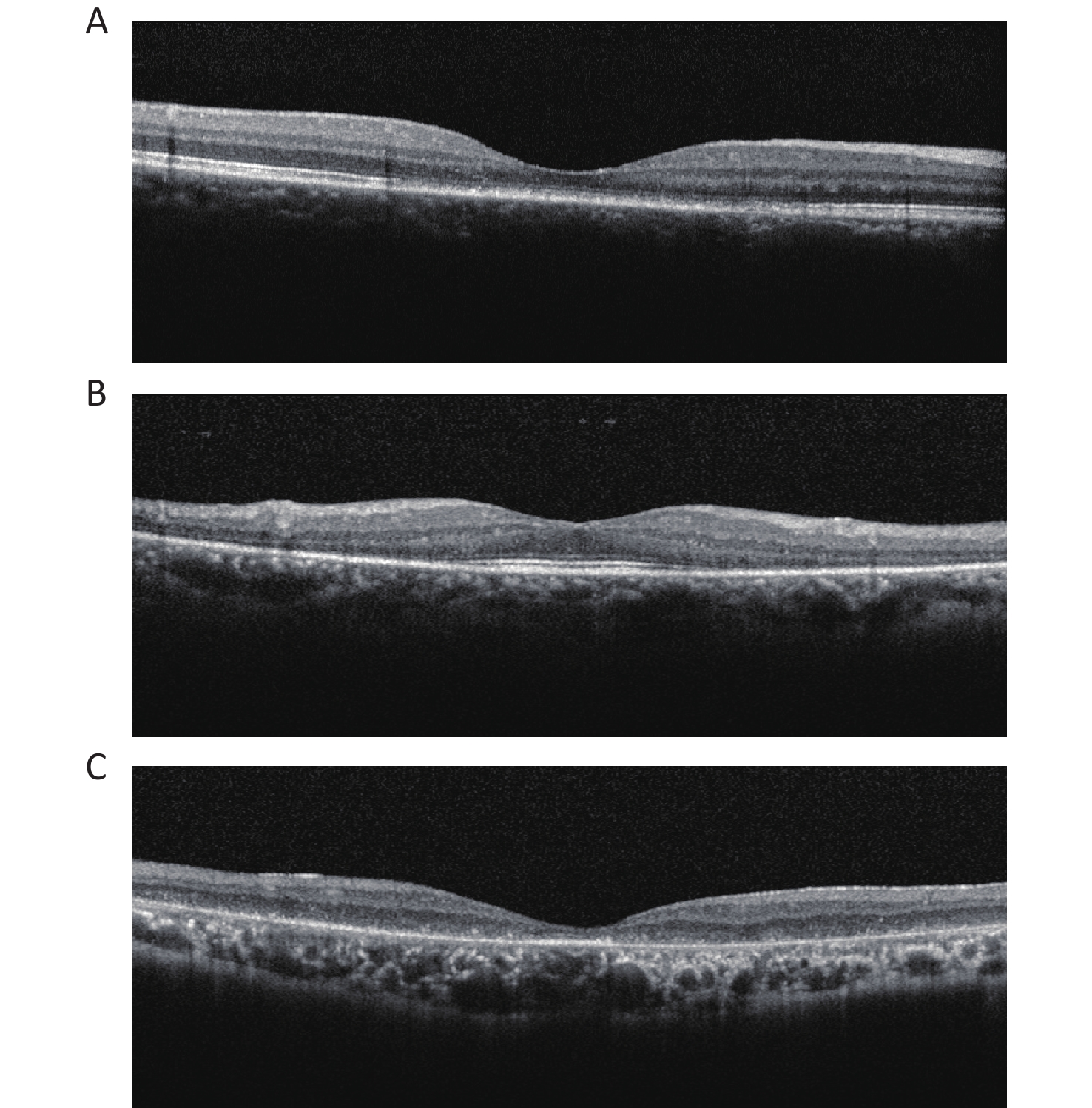
Two certified retinal specialists graded all OCT images in the clinical datasets separately. The diagnosis of IRDs was based on both clinical and genetic detections. The OCT images of IRDs were classified into three types based on morphological features: cone/cone-rod lesions, that is, disruption of photoreceptor layers with thinned sensory retina at the fovea; rod-cone lesions, that is, disruption of photoreceptor layers with thinned sensory retina at the areas outside the fovea with relatively preserved structure at the fovea; and extensive lesions, that is, extensive disruption of photoreceptor layers with thinned sensory retina (Figure 1).

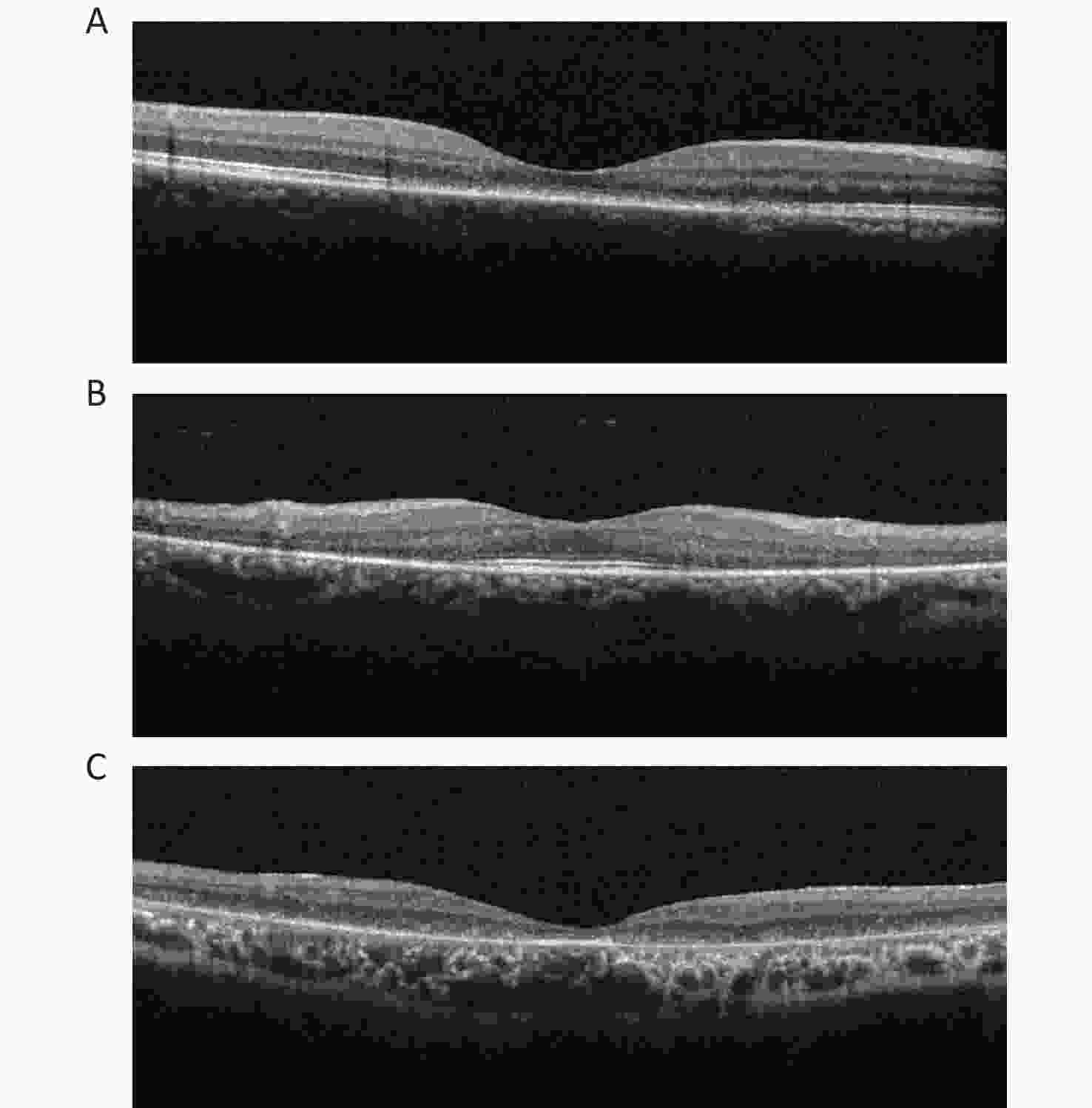
Figure 1.  OCT images of three categories in IRDs. (A) Cone/cone-rod lesions: disruption of photoreceptor layers with thinned sensory retina at the fovea. (B) Rod-cone lesions: disruption of photoreceptor layers with thinned sensory retina at the areas outside the fovea with relatively preserved structure at the fovea. (C) Extensive lesions: extensive disruption of photoreceptor layers with thinned sensory retina. IRDs: inherited retinal disorders.

This study was conducted following the principles of the Declaration of Helsinki. Approval was granted by the Ethics Committee of the Beijing Tongren Hospital, Capital Medical University.

The proposed pipeline consisted of three parts: data preprocessing, training the teacher model, and training the student model. Data preprocessing mainly includes image angle adjustments and vertical pixel column movements. The teacher model was first trained on the auxiliary OCT datasets with a four-class classification designed to learn the nuances of each disease and then transferred to the target OCT dataset to classify the five target classes. The student model was trained using the soft label provided by the teacher model based on knowledge distillation (KD) ^[11] and the hard label from annotation (Figure 2).

Figure 2.  Overview of the proposed method.

The original OCT images show different angles, noise distribution, and size diversity because of the acquisition machine and the patient. This will distract the neural network from the focal area and increase the training time due to useless data input during training. We used a random inversion of the images in the process, which did not destroy the hierarchical information of the OCT images, and cropped the given images to a random size and aspect ratio to increase the generalization ability of the model. The experiments were all preprocessed and resized to 224 × 224 pixels.

The ResNet-50, a convolutional neural network (CNN) framework, was chosen as the teacher model, which is the backbone structure for absorbing and learning the information from the auxiliary dataset, specifically the textures, patterns, and pixel distributions in the end-level convolutional layers. After learning using the same type of dataset, we froze the parameters of the teacher model, except for the last fully connected layer, to transfer the task to the target domain.

To overcome the obstacles caused by the lack of training data, we used the combination of KD and student–teacher learning^[12] for knowledge transfer. ResNet-18 was used as the student model to be trained from scratch to adapt to the target data with a smaller number of samples.

where in Equation 1, α and $\beta $ control the balance of the information coming from the two sources, which generally add up to 1. H is the loss function, σ is the softmax function parameterized by the temperature T, z_s is the logits from the student network, and z_t is the logits from the teacher network. τ denotes the temperature of the adapted softmax function, and each probability p_i of class i in the batch is calculated from logits z_i as follows:

where T in Equation 2 increases, the probability distribution of the output becomes “softer,” which means that the differences among the probabilities of each class decrease and more information will be provided.

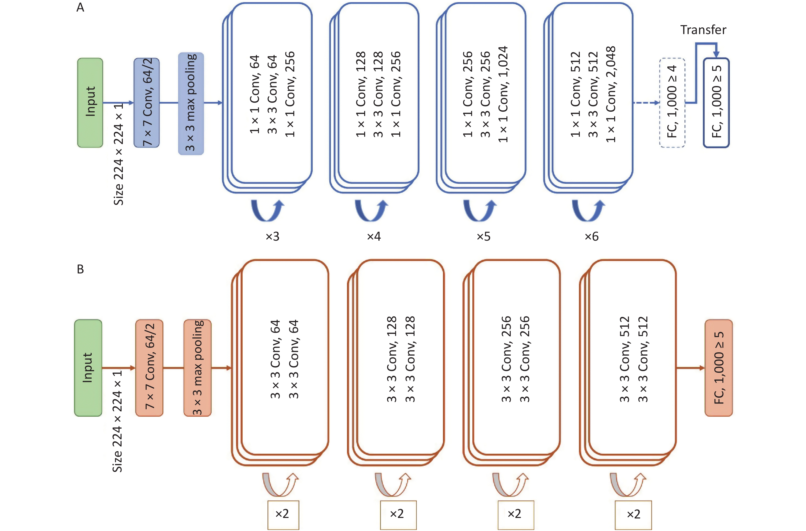
Figure 3 illustrates the network architecture of the model. The model was trained and tested using the Python (version 3.10.7) programming language with the PyTorch (version 1.8.1) library as the backend. The computer used in this study was equipped with an NVIDIA GeForce RTX 2070 8 GB graphics processing unit, 32 GB random access memory, and an Intel Core 11th Gen Intel(R) Core(TM) i9-11900 @ 2.50GHz central processing unit.

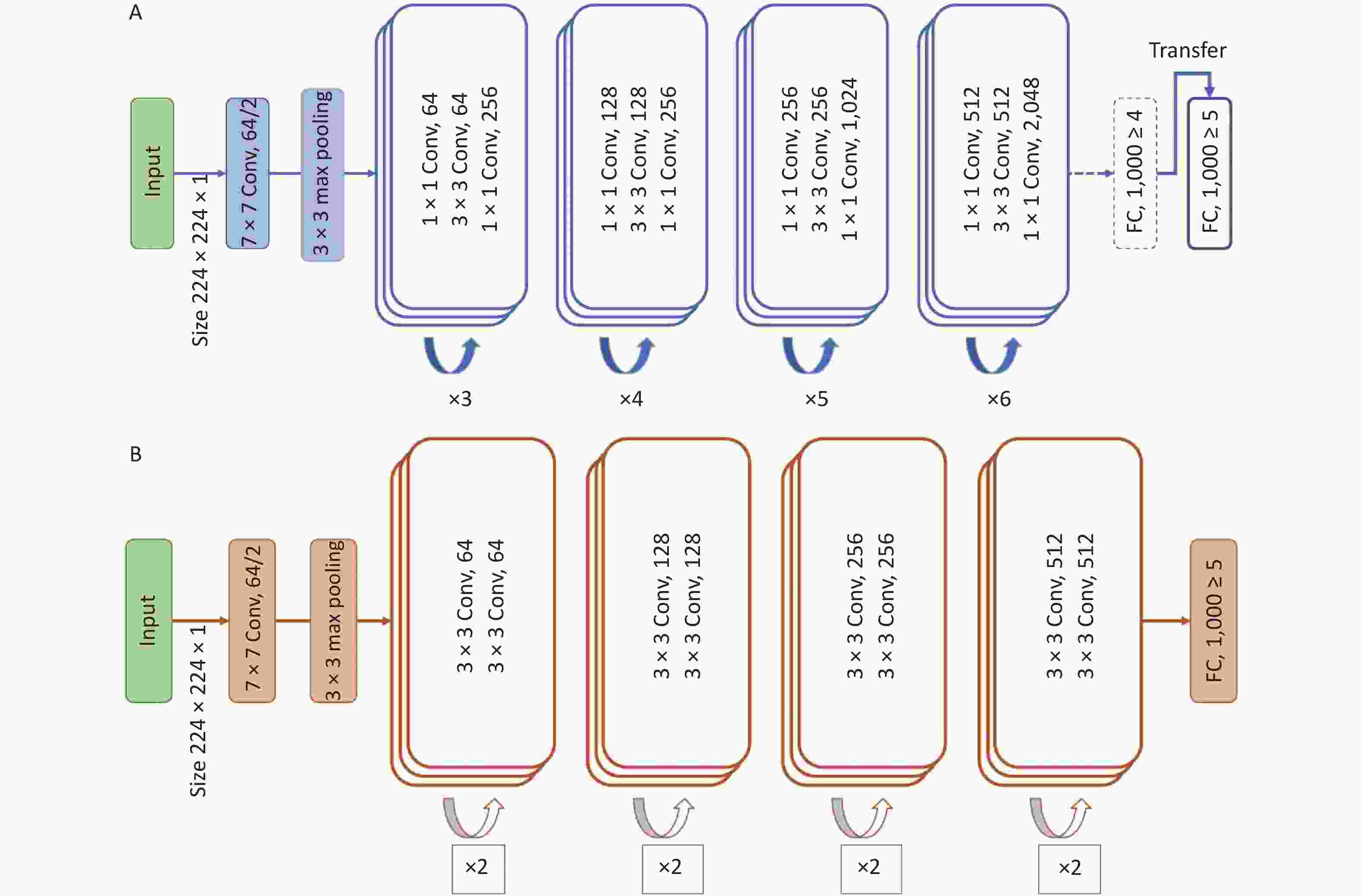
Figure 3.  Network architecture of the model. (A) Teacher model. (B) Student model.

To fully evaluate the performance of the proposed method, we used various evaluation metrics, namely accuracy, sensitivity, specificity, and F1 score, which are defined as follows:

where TP, TN, FP, and FN denote true positives, true negatives, false positives, and false negatives, respectively, and are measured according to the confusion matrix.

Receiver operating characteristic (ROC) curves were also used to display the performance of the FSL model for the classification of OCT images. Heatmaps were used to show the regions of interest (ROI) in the model.

The process was repeated three times with random assignment of participants to the training and testing sets to control for selection bias, given the relatively small sample size. The metrics were calculated for each training/testing process for each category.

A total of 2,317 images from 189 participants were included in this study as the target dataset, of which 1,126 images of 79 participants were IRDs, 533 images of 43 participants were normal samples, and 658 images of 67 participants were controls, including CNV, DME, macular hole, epiretinal membrane, and retinal detachment (Table 1). The images were randomly split in a 3:1 ratio into the training and testing sets.

The FSL model achieved better performance than the baseline model. The baseline model was adapted from ResNet-18, which has the same structure as the student model. The baseline model was added to demonstrate that excluding the advantages of the model performance itself, our proposed method is the main contributor to improving the final results. In the three testing sets, the FSL model achieved a total accuracy ranging from 0.974 [95% confidence interval (CI) 0.968–0.979] to 0.983 (95% CI 0.978–0.987), total sensitivity from 0.934 (95% CI 0.911–0.952) to 0.957 (95% CI 0.936–0.971), total specificity from 0.984 (95% CI 0.978–0.988) to 0.990 (95% CI 0.984–0.993), and total F1 score from 0.935 (95% CI 0.913–0.954) to 0.957 (95% CI 0.938–0.972). The baseline model achieved total accuracy ranging from 0.943 (95% CI 0.934–0.951) to 0.954 (95% CI 0.946–0.961), total sensitivity from 0.866 (95% CI 0.835–0.892) to 0.886 (95% CI 0.856–0.909), total specificity from 0.962 (95% CI 0.954–0.969) to 0.971 (95% CI 0.963–0.977), and total F1 score from 0.859 (95% CI 0.828–0.885) to 0.885 (95% CI 0.857–0.909) (Table 2).

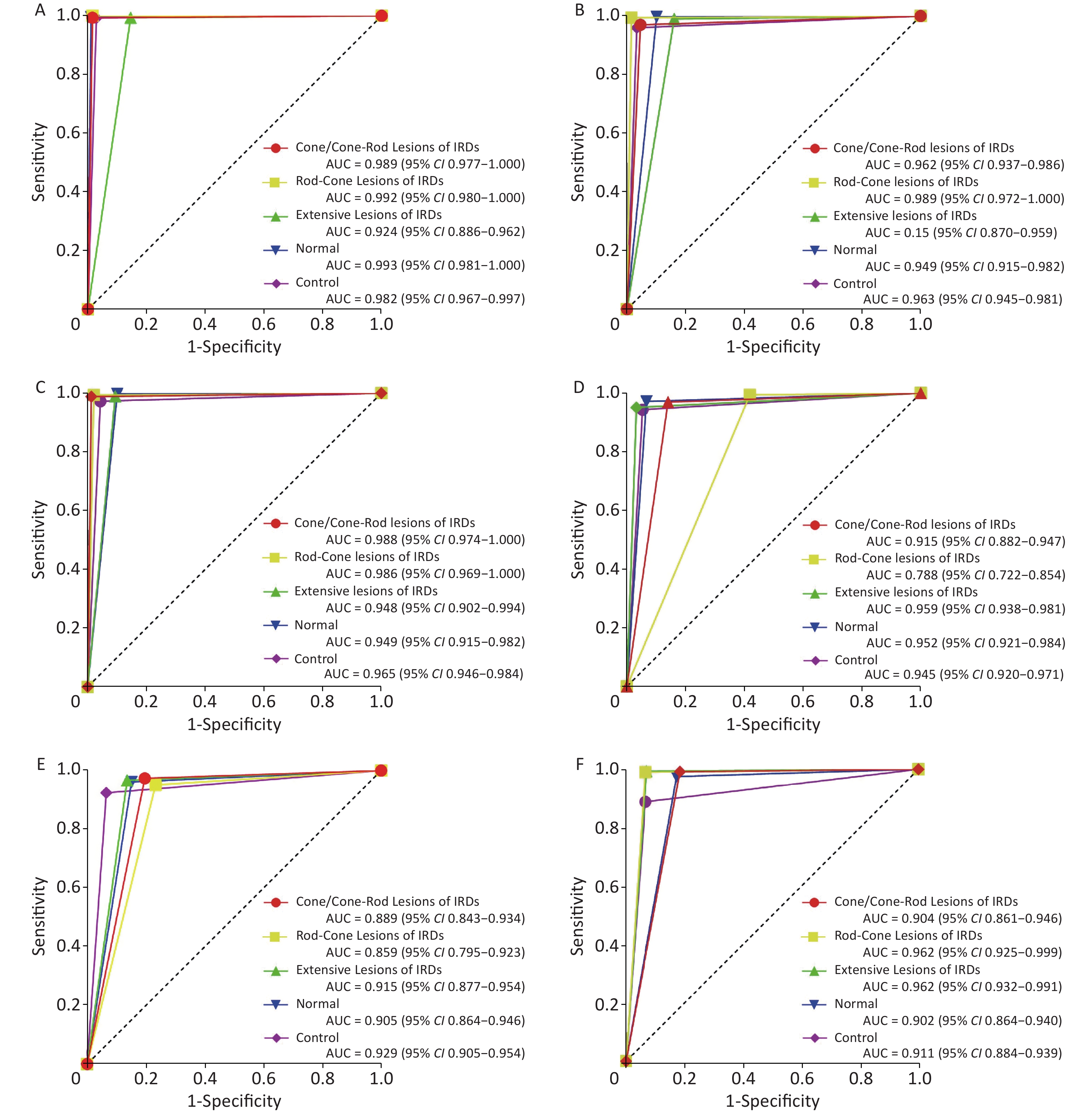
The performance of the FSL model was compared with that of retinal specialists using ROC curve plots. The AUCs of the FSL model were higher for most sub-classifications (Figure 4).

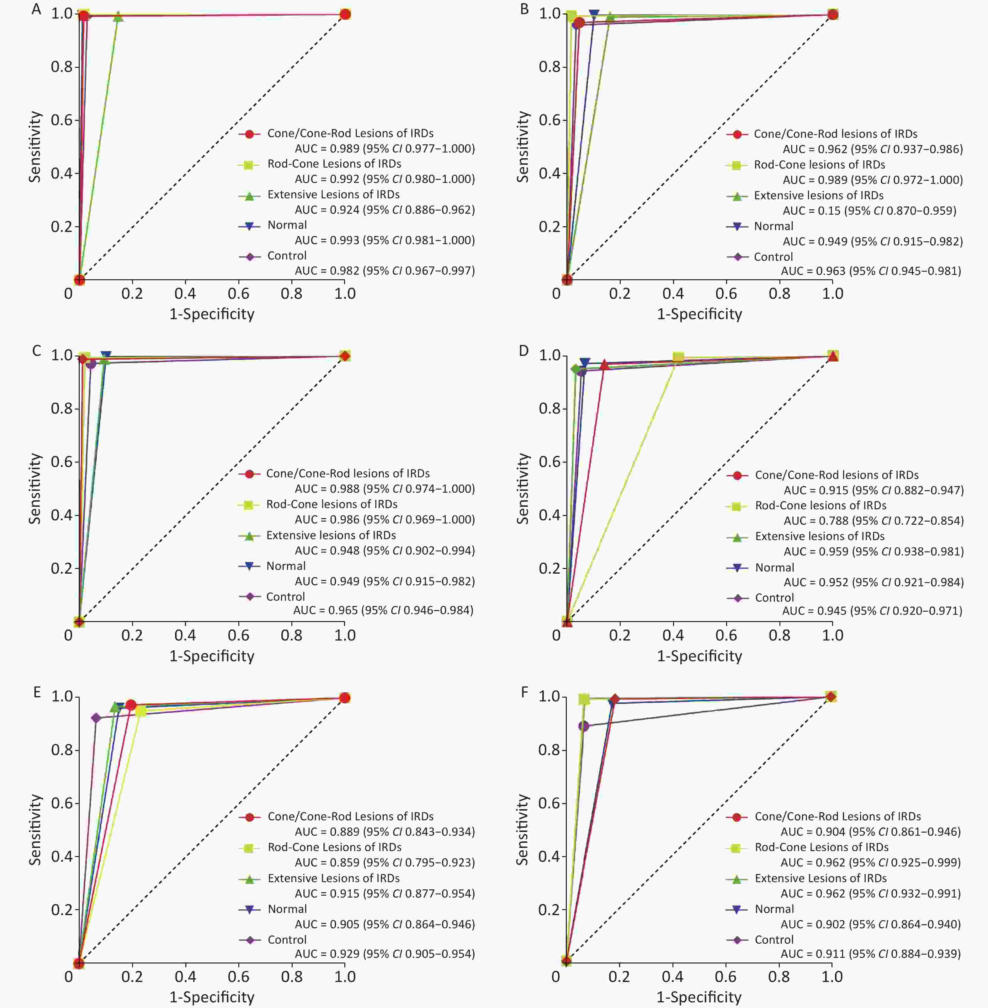
Figure 4.  ROC curves for FSL model and baseline model compared with retinal specialists. (A–C) Test1–3 of FSL model. (D–F) Test1–3 of baseline model. IRDs: inherited retinal disorders; FSL: few-shot learning; AUC: area under curve; CI: confidence interval.

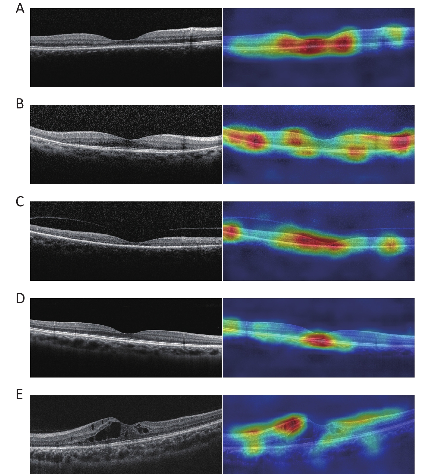
The heatmaps demonstrated that the FSL model made the classification based on the correct lesion for diagnosis (Figure 5).

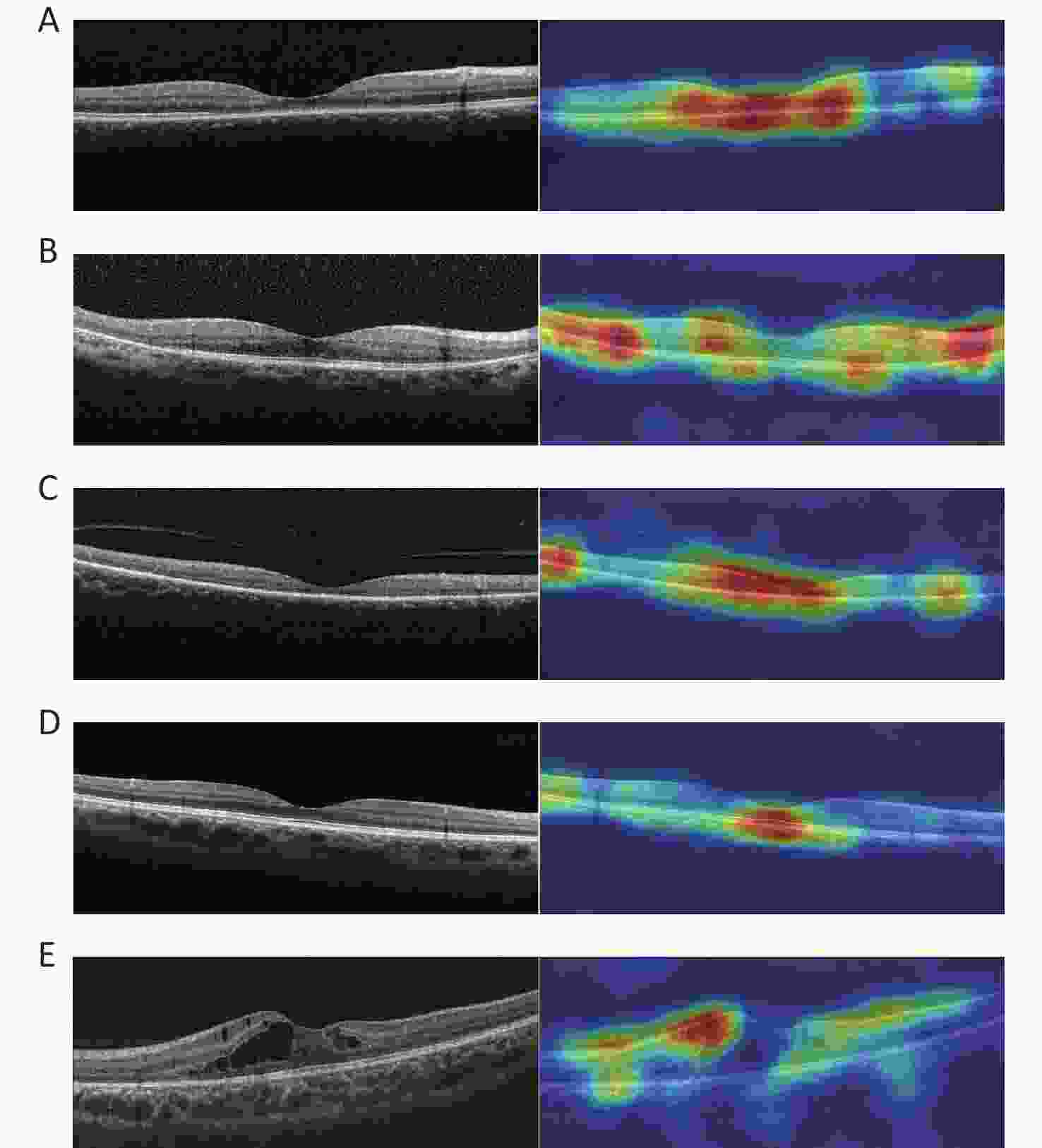
Figure 5.  Representative OCT images and corresponding heatmaps. (A) Example of cone/cone-rod lesions of IRDs and its corresponding superimposed heatmap. (B) Example of rod-cone lesions of IRDs and its corresponding superimposed heatmap. (C) Example of extensive lesions of IRDs and its corresponding superimposed heatmap. (D) Example of normal and its corresponding superimposed heatmap. (E) Example of control and its corresponding superimposed heatmap. IRDs: inherited retinal disorders.

This preliminary study demonstrates the effective use of the FSL model for classifying OCT images from patients with IRDs and normal and control participants with a smaller volume of data.

Previous methods for diagnosing ocular diseases such as AMD and DME through OCT images are based on traditional ML methods such as principal component analysis (PCA)^{[13, 14]}, support vector machine (SVM)^{[10, 15]}, and random forest^[16]. Other studies have focused on DL methods, including improving existing mature and pretrained frameworks, such as Inception-v3^{[17, 18]}, VGG-16^{[17, 19]}, PCANet ^[20], GoogLeNet ^{[21, 22]}, ResNet^{[21, 23]}, and DenseNet^[21] to classify OCT images or unify multiple networks to make the classification more robust for diagnosing, for example, four-parallel-ResNet system^[23] and multi-stage network^[24].

For the success of these algorithms, particularly for tasks such as image recognition, most models are overparameterized to extract the most salient features and ensure generalization. However, the performance of the models is heavily dependent on the very large and high-quality labels of the training datasets. Some studies have reported relevant results. Fujinami-Yokokawa et al.^[25] used Inception-v3 CNN^[26] to classify OCT images from patients with three different IRDs and obtained a relatively high accuracy. Shah et al.^[27] used a new CNN with a simple architecture similar to LeNet^[28], which was more effective than the VGG-19 CNN^[29] in differentiating normal OCT images from images of patients with Stargardt disease. However, varying degrees of overfitting and reduced training accuracy were observed. These are the disadvantages of large DL algorithms for small sample data.

Traditional network frames and large-volume data are no longer suitable for identifying rare diseases, such as IRDs, that belong to the small-sample classification problem. Therefore, the concept of FSL has been proposed to solve such problems^{[30, 31]}. FSL combines limited supervision information (small samples) with prior knowledge (unlabeled or weakly labeled samples, other datasets and labels, other models, etc.) such that the model can effectively learn information from small samples. Recently, a few FSL methods, such as contrastive self-supervision learning^[32], generative adversarial networks (GAN)^[33], integrated frameworks ^[34], and unsupervised probabilistic models ^[35], have been used for the segmentation and classification of fundus images.

This is the first time that FSL has been used to classify OCT images of IRDs. Our model is based on a student–teacher learning framework, an appealing paradigm for semi-supervised learning in medical image classification. The images were normalized using conventional preprocessing to reduce the effect of noise on the model during training. The teacher model is designed to adapt to the target dataset based on TL^[36], an approach to increase the performance of DL classifiers, in which a large multiclass image classifier is pretrained on a natural image dataset and then retrained on the smaller medical imaging dataset of interest. The resulting model has fewer parameters to be trained than the original model and is “fine-tuned” for the medical imaging task. In the process from the teacher model to the student model, the KD method^[11] that we chose was soft-target training in which the teacher generates soft labels^[37] for the training data, and these soft targets are used in combination with one-hot encoded labels (hard targets) to train the student model. KD refers to a method that helps the training process of a smaller student network under the supervision of a larger teacher network. Unlike other compression methods, KD can downsize a network regardless of the structural difference between the teacher and student networks ^[12]. With this framework, the student model could increase the training speed, prevent overfitting, result in more generalized models, and maintain a relatively simple structure simultaneously.

Our FSL model attained higher total accuracy, sensitivity, specificity, and F1 score than the baseline model and achieved better performance for most subclassifications. The differences in the sensitivity and F1 scores between the two models were more apparent. Higher sensitivity demonstrated that the model could achieve better classification results. Moreover, the F1 score is the harmonic mean of precision and recall, indicating the robust performance of the model. In addition, an interesting phenomenon exists, in which the specificity of both models was greater than the sensitivity, suggesting that the classification of models tended to be conservative. This may also be more secure for potential clinical applications. The ROC analysis also showed that the FSL model had higher AUCs for most subclassifications. The heatmaps demonstrated that the regions highlighted with warmer colors represented areas more critical for final class determination. The ROIs were precisely captured by the FSL model, and the results were compatible with the judgment of the retinal specialist. In this study, we trained and tested OCT images from different devices and sizes, and proved that the model had good generalizability. In summary, our FSL model could perform comparably to the advanced large teacher model and in a fraction of the time, making ideal candidates run in clinical settings where the runtime is important, and computing resources are often limited.

Several recent studies have reported that the combination of multiple modalities and imaging techniques can improve diagnostic performance. Yoo et al.^[38] designed an algorithm based on the combination of fundus photographs and OCT images, which increased the diagnostic accuracy of AMD compared with the data alone. Miri et al.^[39] used complementary information from fundus photographs and OCT volumes to segment the optic disc and cup boundaries. Fundus and OCT images are recognized as the most influential biomarkers of retinal diseases. However, previous studies have paid little attention to the function of a diagnostic model that combines the fundus with OCT images. Images from different devices can provide unique and complementary information. Our study needs to adopt a multimodal process to combine various types of imaging for a more precise performance in the future.

This study had some limitations. The clinical datasets included only patients with a sample size, which led to the existence of a potential similarity in the case of multiple images from the same patient. Future research, including genetic data with sufficient patient numbers to represent the significant phenotypic and genetic heterogeneity of IRDs, may help with phenotype–genotype correlation. Second, the cross-sectional study could not identify the sequence of intraretinal structural changes in the transitional zone over time, and misclassification due to disease progression may occur. Incorporating temporal data into the model may allow the leading disease front to be automatically identified and monitored.

In this preliminary study, we demonstrated the potential of the FSL model to differentiate OCT images of IRDs from healthy individuals and patients with other common macular diseases. Furthermore, the model can also distinguish between different types of IRDs using a dataset smaller than that traditionally used. In real-life clinical settings, the general principle demonstrated in this study and similar network architectures can be applied to other retinal diseases with a low prevalence.

The authors have no conflict of interest to declare.