Prediction of Renal Function by Urinary Lead and Cadmium — Based on Classification Decision Tree and Logistic Regression Model

It is estimated that chronic kidney disease (CKD) will be the fifth leading cause of death in the world by 2040^[1]. Early recognition and intervention for kidney damage are essential. Estimated glomerular filtration rate (eGFR) can be calculated by measuring blood creatinine to evaluate glomerular function, and urinary N-acetyl-β-δ-glucosaminidase (UNAG) level is generally recognized as a marker of renal tubular injury. Exposure to lead (Pb) and cadmium (Cd) can damage renal function, leading to a decrease in eGFR and an increase in UNAG^[2]. Both Pb and Cd are easily accumulated in the body and then slowly released by the kidneys and excreted. So, urinary Pb (UPb) and Cd (UCd) levels can be used as biomarkers of exposure^[3,4]. Therefore, predicting renal function based on UPb and UCd levels may provide scientific evidence for establishing toxicity thresholds and provide reasonable strategies for preventing kidney damage. Logistic regression and classification decision tree are commonly used as predictive models to identify the factors that affect diseases^[5]. The logistic regression combined with classification decision tree models to predict renal impairment is currently lacking. In this study, eGFR and UNAG were used as effect indicators, and UPb and UCd levels were included as factors in the prediction model, to construct logistic regression and classification decision tree model, and analyzed the predictive performance of the model.

This study is a community-based cross-sectional survey in which we randomly selected residents from two communities in northern China as study participants through whole population sampling. The inclusion criteria for this study were as follows: age over 18 years, residing locally area for at least 5 years, and voluntarily participating in the survey. The exclusion criteria included individuals with secondary kidney diseases such as diabetic nephropathy, those taking medications that could affect renal function, occupationally exposure to heavy metals, and those with insufficient information or incomplete samples. Baseline information on the study participants was collected including gender, age, education level, per capita monthly household income, smoking, and alcohol consumption. The physical examination included height and weight, and the body mass index (BMI) was calculated based on height and weight. Urine specimens were collected from the study participants to measure urinary creatinine (UCr), UCd, UPb, and UNAG. And UCr levels were used to correct for urinary heavy metal levels and UNAG. Blood samples were collected from the study participants to measure high-density lipoprotein cholesterol (HDLC), total cholesterol (TC) levels, and serum creatinine (SCr), and SCr was used to calculate the eGFR. Dual data entry using EpiData version 3.0 to create the database. Divided the dataset into training and testing set in a ratio of 7:3. Before building the model, univariate analysis was performed by SPSS 26.0 software with eGFR and UNAG as dependent variables, respectively. Study participants were divided into a low eGFR group (eGFR ≤ 60.00 mL/min per 1.73 m²) and a control group (eGFR > 60.00 mL/min per 1.73 m²) based on clinically recognized eGFR diagnostic thresholds^[6]. Divided into a high UNAG group (UNAG ≥ 16.28 U/g Cr) and a UNAG control group (UNAG < 16.28 U/g Cr) according to the median level of UNAG (16.28 U/g Cr). Statistically significant independent variables were included in logistic regression and classification decision tree. The variance inflation factor (VIF) was utilized to test for the multicollinearity between variables. R4.0.4 software was used to construct the model on the training set, and the predictive performance of the model was assessed by creating participant’s working characteristic curve (receiver operating characteristic) and confusion matrix, calculating the area under the curve, sensitivity, specificity, accuracy, and precision. Two-sided P values < 0.05 were statistically significant.

Based on the inclusion and exclusion criteria, 532 participants were included in our study, of which 190 were males and 342 were females. The differences in per capita monthly household income, smoking and alcohol consumption were statistically significant between males and females. Further details on participant characteristics are shown in Supplementary Table S1 (available in www.besjournal.com). The results of univariate analysis showed that there were statistically significant differences (P < 0.001) between the low eGFR and the eGFR control groups in terms of gender, age, education level, per capita monthly income, alcohol consumption, TC/HDL ratio, UCd, and UPb levels (Supplementary Table S2, available in www.besjournal.com). And there were statistically significant differences between the high UNAG and the UNAG control groups in terms of age (P < 0.001), education (P < 0.001), UCd (P < 0.001), and UPb (P = 0.018) levels (Supplementary Table S3, available in www.besjournal.com). The variable assignments for the logistic regression are shown in Table 1, and the VIF for all variables were less than 5, indicating a low likelihood of multicollinearity among the variables in the model (Supplementary Tables S4–S5, available in www.besjournal.com).

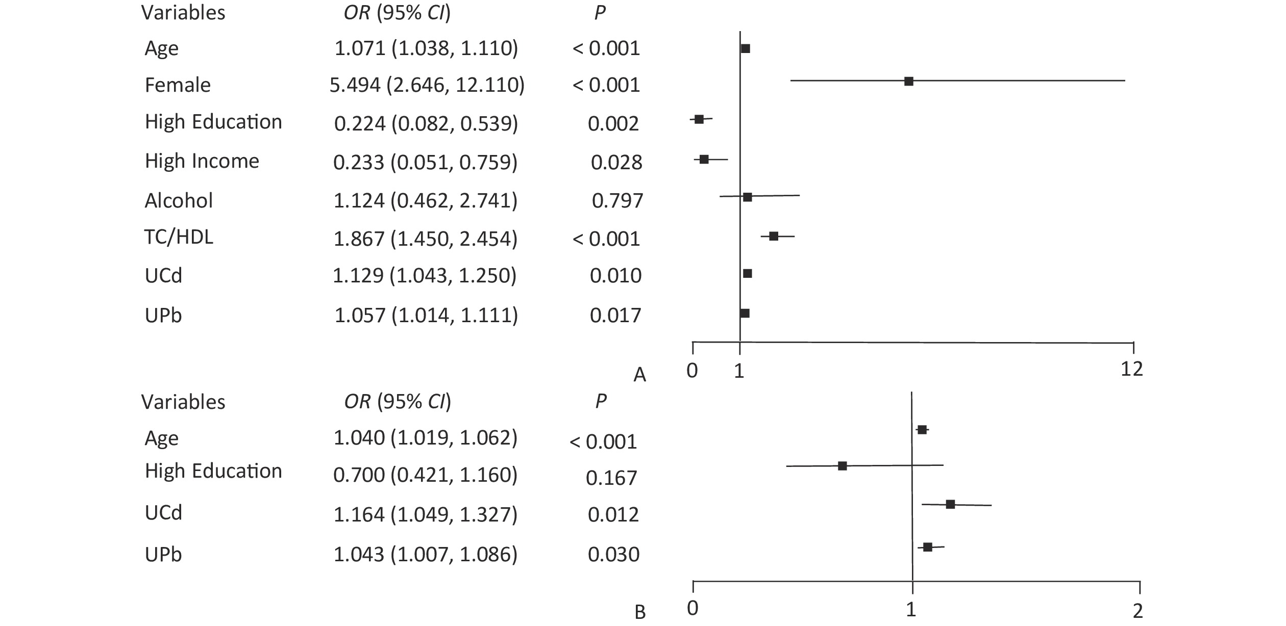
The node variables included in the classification decision tree have both differences and similarities with the significant variables in logistic regression. The logistic regression results showed that UPb and UCd levels were risk factors for low eGFR (Figure 1A) and high UNAG (Figure 1B). The classification decision tree results showed the same results, with UPb level being the best classified feature for predicting the eGFR (Figure 2A) and UCd level being the best classified feature for predicting high UNAG (Figure 2B). Older age is also a risk factor for low eGFR and high UNAG (Figures 1–2), this is probably because renal function gradual decline with age, and changes in the structure and function of the kidneys, such as renal arteriosclerosis, glomerulosclerosis, and renal tubular atrophy with fibrosis^[7]. When predicting eGFR, both logistic regression and classification decision tree incorporated the variables such as female and TC/HDL, suggesting that both female and TC/HDL levels were risk factors for lower eGFR (Figure 1A and Figure 2A), probably because the average age of the study participants in this study being around 60 years old, and it has been shown that a significant decrease in estrogen levels in older women lead to a decrease in the protective effect of the vascular endothelial system, resulting in a significant decrease in eGFR^[8]. It has also been shown that lower TC and higher HDL levels are associated with a lower incidence of CKD, lower TC levels and higher HDL levels may have a protective effect on the kidneys^[9]. However, logistic regression showed higher OR for female and TC/HDL (Figure 1A), suggesting that females and those with higher levels of TC/HDL are at greater risk of developing lower eGFR. In the classification decision tree, the two characteristic variables of female and TC/HDL level, were classified as leaf nodes rather than root node, with the root node was UPb level (Figure 2A). In addition, the logistic regression results also showed that higher income level and higher education level were protective factors for eGFR (Figure 1A), which may be due to the association between higher income and higher education level and better health management, which were not taken into account in the final classification decision tree model (Figure 2A). The similarities and differences between logistic regression and classification decision trees may be due to the different focuses of the two models. Logistic regression is a linear model that predicts outcomes by fitting a linear relationship to the data, focuses on explaining how the probability of the dependent variable changes when the independent variable changes. Its main purpose is to explore the risk factors of diseases and predict the probability of of disease occurrence based on risk factors. In contrast, the classification decision tree is a nonlinear model that divides the data based on the values of the predictors, focuses on classifying all samples into the closest category by selecting the appropriate dividing characteristics at each node. Classification decision trees are able to find the optimal cutoff point for successive predictors in logistic regression. Both logistic regression and classification decision tree are more commonly used to categorize and predict models for dichotomous variables. In practice, the performance of these two models on a given dataset can be compared to determine which model is more suitable for a particular task, and the two models are used for different purposes and can be combined in practice to improve analytical performance.

Figure 1.  Forest plot of eGFR and UNAG impact factors. (A) Forest plot of eGFR influencing factors; (B) Forest plot of UNAG influencing factors; eGFR, estimated glomerular filtration rate; UNAG, urinary N-acetyl-β-δ-glucosaminidase; HDL, high-density lipoprotein cholesterol; TC, total cholesterol; UCd, urinary cadmium; UPb, urinary lead.

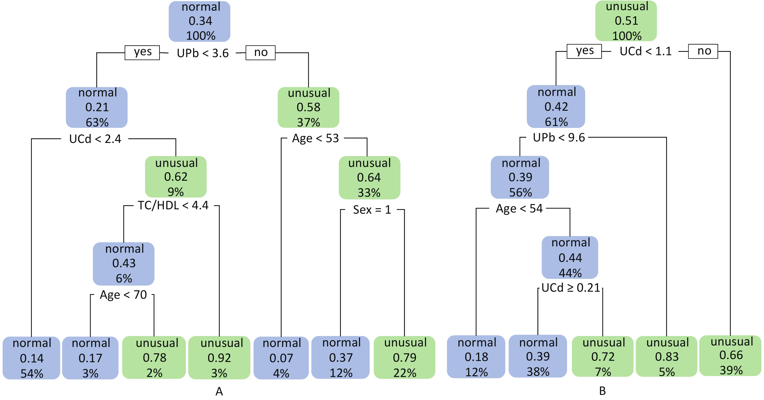
Figure 2.  Classification decision trees for eGFR and UNAG. (A) Classification decision tree with eGFR as dependent variable; (B) Classification decision tree with UNAG as dependent variable; Blue leaf nodes indicated the probability that ≤ 50% of study participants have lower eGFR and higher UNAG, defined as normal eGFR and normal UNAG. Green leaf nodes indicate the probability that > 50% of study participants have lower eGFR and higher UNAG, defined as abnormal eGFR and abnormal UNAG. Decimal points indicate the probability that the classified population has lower eGFR and higher UNAG. Percentages indicate the percentage of the training set sample size that this categorized population represents. eGFR, estimated glomerular filtration rate; UNAG, urinary N-acetyl-β-δ-glucosaminidase; HDL, high-density lipoprotein cholesterol; TC, total cholesterol; UCd, urinary cadmium; UPb, urinary lead.

The final model of the eGFR classification decision tree showed a 79% probability of lower eGFR in women aged over 53 years and had the UPb level ≥ 3.60 μg/g Cr. And a 92% probability of lower eGFR if the UPb level was < 3.60 μg/g Cr, the UCd level was ≥ 2.40 μg/g Cr, and the TC/HDL ratio was ≥ 4.4. The probability of low eGFR was 78% if the age was ≥ 70, the UPb level was < 3.60 μg/g Cr, the UCd level was < 2.40 μg/g Cr, and the TC/HDL ratio was < 4.4. (Figure 2A). The final UNAG classification decision tree results show that if the UCd level was ≥ 1.10 μg/g Cr, the probability of higher UNAG level was 66%; if the UCd level was < 1.10 μg/g Cr and the UPb level was ≥ 9.60 μg/g Cr, the probability of higher UNAG level was 83%; and if the UCd level was < 0.21 μg/g Cr , the UPb level was < 9.60 μg/g Cr, and the age was not less than 54 years, the probability of having a higher UNAG level was 72% (Figure 2B). And when the predictive variables were ranked by importance, UPb and UCd levels were the top two variables (Supplementary Figures S1–S2, available in www.besjournal.com), suggesting that reducing Pb and Cd exposure is more important than lowering the TC/HDL ratios or increasing education and income levels to protect kidney function. In addition, in this study population, the probability of eGFR abnormality was 14% when the UPb level was < 3.60 μg/g Cr and the UCd level < 2.40 μg/g Cr (Figure 2A). When the UCd level was < 1.10 μg/g Cr, the UPb level was < 9.60 μg/g Cr, and the age was less than 54 years, the probability of UNAG abnormality was 18% (Figure 2B). Suggest that kidney damage is possible when UCd level is > 1.10 μg/g Cr or UPb level is > 3.60 μg/g Cr, this indicates that UCd levels below the toxicity threshold levels recognized by the World Health Organization (5.24 µg/g Cr) may also trigger body damage^[10]. For renal impairment, the toxicity threshold level of UPb could be < 3.60 μg/g Cr.

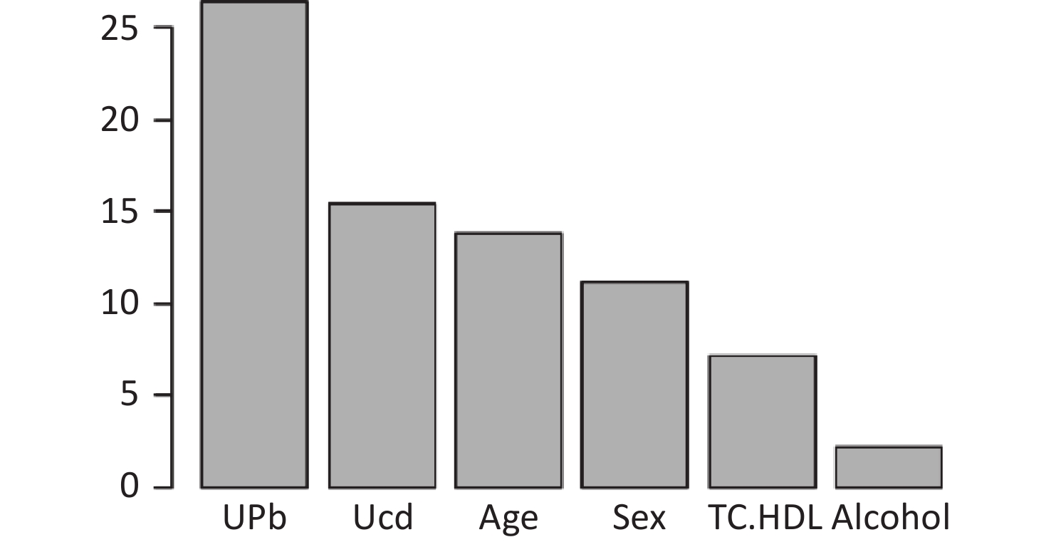
Figure S1.  Ranking of the Importance of Risk Factors for estimated glomerular filtration rate (eGFR). Using eGFR as a renal function indicator, UPb and UCd levels are more important predictive variables. eGFR, estimated glomerular filtration rate; HDLC, high-density lipoprotein cholesterol; TC, total cholesterol; UCd, urinary cadmium; UPb, urinary lead.

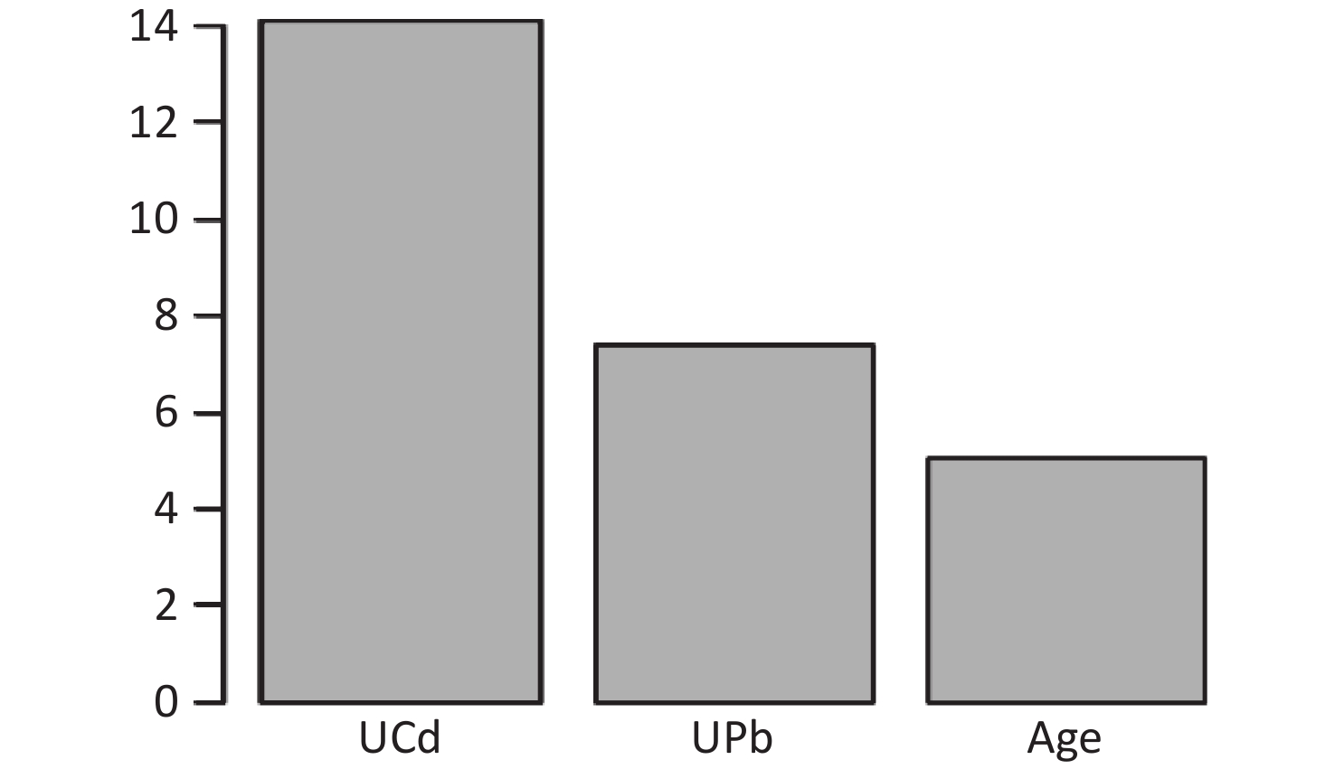
Figure S2.  Ranking of the Importance of Risk Factors for urinary N-acetyl-β-δ-glucosaminidase (UNAG). Using UNAG as a renal function indicator, UCd and UPb levels are more important predictive variables. UCd, urinary cadmium; UPb, urinary lead.

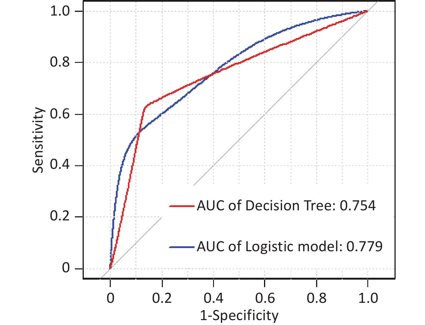
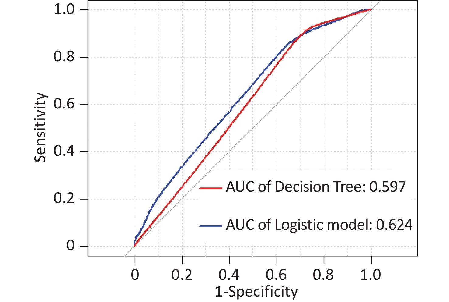
In this study, area under the curve, sensitivity, specificity, accuracy, and precision were calculated using ROC curves and confusion matrices, respectively, to assess the predictive performance of the models. eGFR was used as the effect indicator, the area under the ROC curve for the logistic regression and classification decision tree models were 0.779 (95% CI: 0.709–0.844) and 0.754 (95% CI: 0.697–0.844) (Supplementary Figure S3, available in www.besjournal.com). The sensitivity, specificity, precision, and accuracy of the logistic regression model were 56.1%, 84.5%, 66.7%, and 74.4% (Supplementary Figure S4A, available in www.besjournal.com), respectively, as well as the sensitivity, specificity, precision, and accuracy of the classification decision tree were 62.9%, 86.7%, 75.0% and 77.5% (Supplementary Figure S4B). And using UNAG as the effect indicator, the logistic regression model and the classification decision tree model showed that the area under the ROC curve were 0.624 (95% CI: 0.543–0.702) and 0.597 (95% CI: 0.53–0.675) (Supplementary Figure S5, available in www.besjournal.com). The logistic regression model had a sensitivity, specificity, precision, and accuracy of 50.7%, 56.6%, 56.1% and 58.1%, respectively (Supplementary Figure S6A, available in www.besjournal.com). The classification decision tree had a sensitivity, specificity, precision, and accuracy of 53.3%, 57.7%, 55.6% and 52.6%, respectively (Supplementary Figure S6B). The area under the ROC curve of both models was greater than 0.5, and the confusion matrix also showed that the sensitivity, specificity, precision and accuracy of both models were higher than 50%. It indicated that both models have certain predictive performance, and UPb levels and UCd levels can be used as indicators to predict lower eGFR and higher UNAG levels.

Figure S3.  Receiver operating characteristic (ROC) curve of the eGFR prediction model. The AUCs were all greater than 0.5, indicating that the model evaluation was effective. AUC, area under the curve; ROC, receiver operating characteristic; eGFR, estimated glomerular filtration rate.

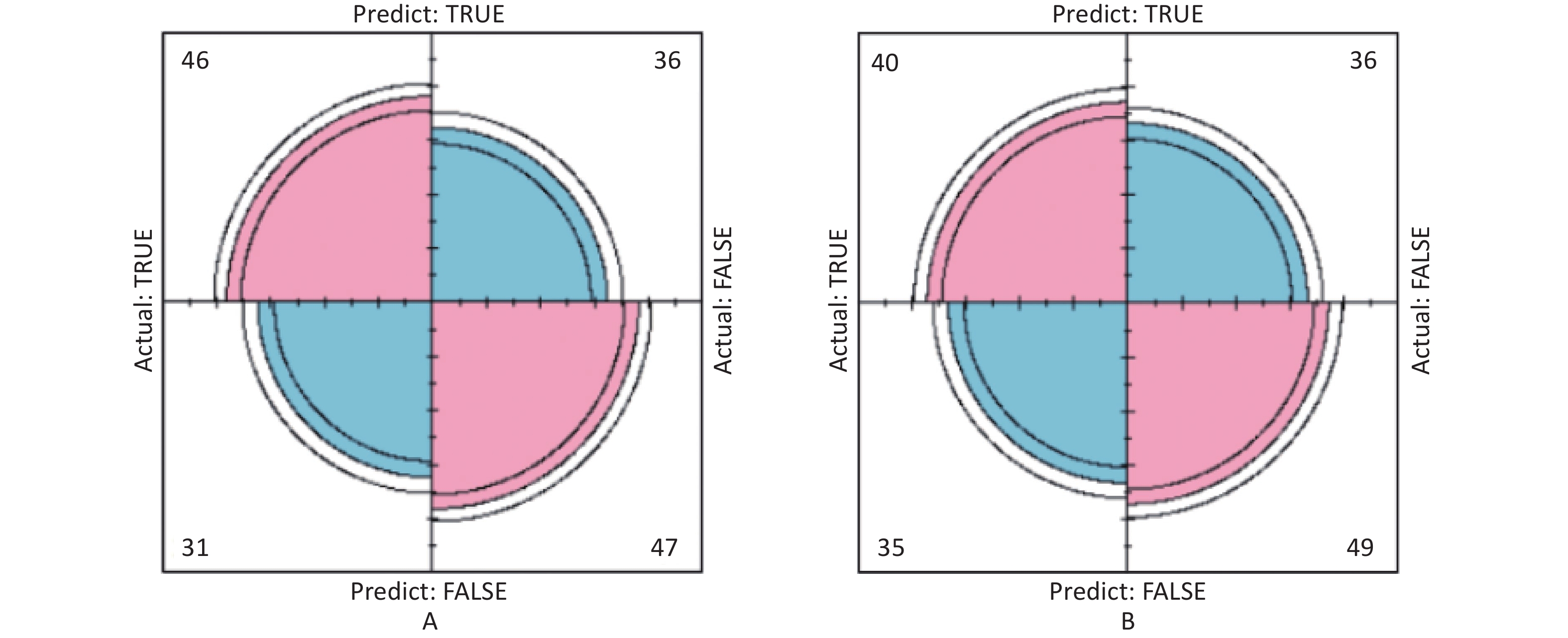
Figure S4.  The prediction model confusion matrix of eGFR. (A) Confusion matrix for eGFR logistic regression; (B) Confusion matrix for eGFR classification decision tree. The pink part in the figure represents the correct prediction and the blue part represents the incorrect prediction. With eGFR as an indicator of renal function, classification decision tree models have higher sensitivity, specificity, precision and accuracy than logistic regression (True positive is shown by the number in the upper left corner, false positive is shown by the number in the upper right corner, false negative is shown by the number in the lower left corner, and true negative is shown by the number in the lower right corner). eGFR, estimated glomerular filtration rate.

Figure S5.  Receiver operating characteristic (ROC) curve of the UNAG prediction model. The AUCs were all greater than 0.5, indicating that the model evaluation was effective. AUC, area under the curve; ROC, receiver operating characteristic; UNAG, urinary N-acetyl-β-δ-glucosaminidase

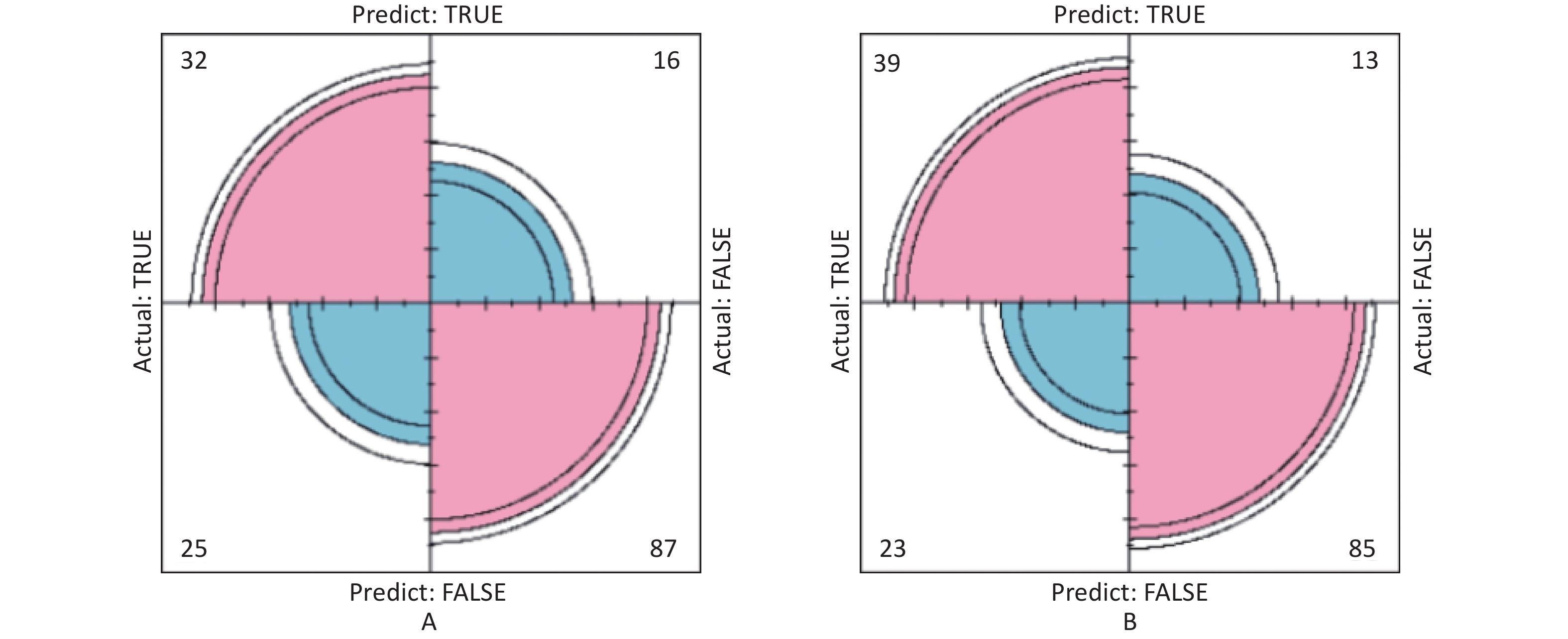
Figure S6.  Confusion matrix of UNAG prediction model. (A) Confusion matrix for UNAG logistic regression; (B) Confusion matrix for UNAG classification decision tree. The pink part in the figure represents the correct prediction and the blue part represents the incorrect prediction. With UNAG as the indicator of renal function, the sensitivity and specificity of the classification decision tree model are higher than those of the logistic regression (True positive is shown by the number in the upper left corner, false positive is shown by the number in the upper right corner, false negative is shown by the number in the lower left corner, and true negative is shown by the number in the lower right corner). UNAG, urinary N-acetyl-β-δ-glucosaminidase

In this study, using cross-sectional data to construct the model has certain advantages. Firstly, the sample data can be obtained and the relationship between the variables can be evaluated in a shorter time. Secondly, the model constructed from cross-sectional data requires fewer parameters, which reduces the complexity of the model and the probability of error. This study also has some limitations. Firstly, participants were recruited from two selected random communities in Taiyuan, Shanxi Province, China. Therefore, to confirm the generalizability of these results, similar studies should be conducted in other regions. Secondly, because our study was a cross-sectional study, causality could not be established. The effect of UPb and UCd levels in predicting impaired renal function needs to be verified through cohort studies. This study only uses internal validation and only tests the model’s ability to predict sample data, and these results require further external validation.

In conclusion, we found that high levels of UPb and UCd, as well as older age, were associated with lower eGFR and higher UNAG. In this study, the UPb level was the best predictor of lower eGFR, while the UCd level was the best predictor of higher UNAG level. The ROC curves and confusion matrixes showed that the constructed model had good predictive performance. These results provide a potential scientific research basis for predicting renal function based on UPb and UCd levels, which may provide new research directions for the early diagnosis of kidney diseases.

We would like to thank all the study participants who volunteered to take part and all the community workers for their support of our research work.

The authors declare that they have no conflict of interest.