Scarlet fever (SF) is a common infectious disease caused by group A streptococcus (GAS)^[1]. During the 18th and 19th centuries, SF was a significant cause of mortality in children aged 5–15 years worldwide^[2]. The incidence and fatality rates of SF have decreased remarkably due to the widespread use of effective antibiotics and improvements in diet and sanitation^[3]. However, the recent resurgence of SF has sparked significant interest in infectious diseases^[1,3]. Given the insufficient understanding of the triggers that cause SF outbreaks and the absence of available vaccines to prevent GAS infection to date^[1], effective prevention and control programs are needed to manage the ongoing spread of SF.

Time-series analysis is an invaluable tool for decision-making and strategic planning because of its ability to uncover patterns, trends, and relationships by examining and interpreting data points collected over a period^[4]. Seasonal autoregressive integrated moving average (SARIMA) is the most common model in the field of health because of its straightforward structure, rapid applicability, and ability to provide meaningful insights into datasets^[4]. SARIMA has proven successful in estimating the prevalence, morbidity, and mortality of contagious diseases. This is achieved by capturing temporal dependency properties and accounting for changing trends, periodic fluctuations, and random variations in a time series^[4,5]. However, SARIMA fails to capture long-term temporal dependencies because it is designed to model short-term fluctuations. Moreover, the use of integer differencing in SARIMA can lead to over-differencing, potentially removing valuable information that can affect parameter estimation and fitting. Conversely, the seasonal autoregressive fractionally integrated moving average (SARFIMA), which incorporates fractional differencing into SARIMA, overcomes these limitations^[6]. Thus, it is well-suited for analyzing both short- and long-term memory in time series, such as finance, economics, hydrology, and meteorology^[6]. Additionally, SARFIMA does not involve complex mathematical concepts. This transparency enables end users to understand how the model is built and to depend more on the results for decision-making purposes. Despite these promising attributes, no published work has been conducted using this method to analyze and evaluate SF epidemics. Therefore, the objectives of this study were to examine the flexibility and efficacy of SARFIMA in estimating SF epidemics in Liaoning, where the yearly average morbidity was 10.363 per 100,000 persons, which is significantly higher than the average level (average, 3.26 per 100,000 people per year) in China^[7]. This study also aimed to compare the predictive accuracy and reliability of SARFIMA against SARIMA.

We retrospectively gathered monthly SF incident cases and population data of Liaoning between January 2004 and December 2019 from the National Notifiable Infectious Disease Surveillance System and the Statistical Yearbook. Subsequently, the series was split into two segments: a training subset from January 2004 to December 2018 to establish the SARIMA and SARFIMA and a test subset from January to December 2019 to validate the generalization of the models. An additional testing dataset from January 2004 to December 2017 was used to determine the reliability of the models. The trend, seasonal, and irregular components were estimated using Seasonal and Trend decomposition with the Loess technique. The seasonal relative, indicating the amount by which the incidence for that specific time tended to be higher (or lower) than the average, was computed using multiplicative decomposition. Changing SF epidemic patterns were estimated using the average annual percentage change (AAPC) based on Joinpoint (version 4.8.0.1). SARIMA and SARFIMA were created using the “forecast” and “arfima” packages in R 4.2. Moreover, the incidence rate ratio (IRR) with a 95% confidence interval (CI) was computed in the pre- and post-outbreak SF by comparing the two proportions^[2]. To determine the predictive quality, two types of measurement indicators were calculated: scale-dependent metrics, such as mean absolute deviation (MAD) and root mean square error (RMSE), and metrics based on percentage errors, such as mean absolute percentage error (MAPE), mean error rate (MER), and root mean square percentage error (RMSPE)^[5]. A better model was developed by minimizing these metrics.

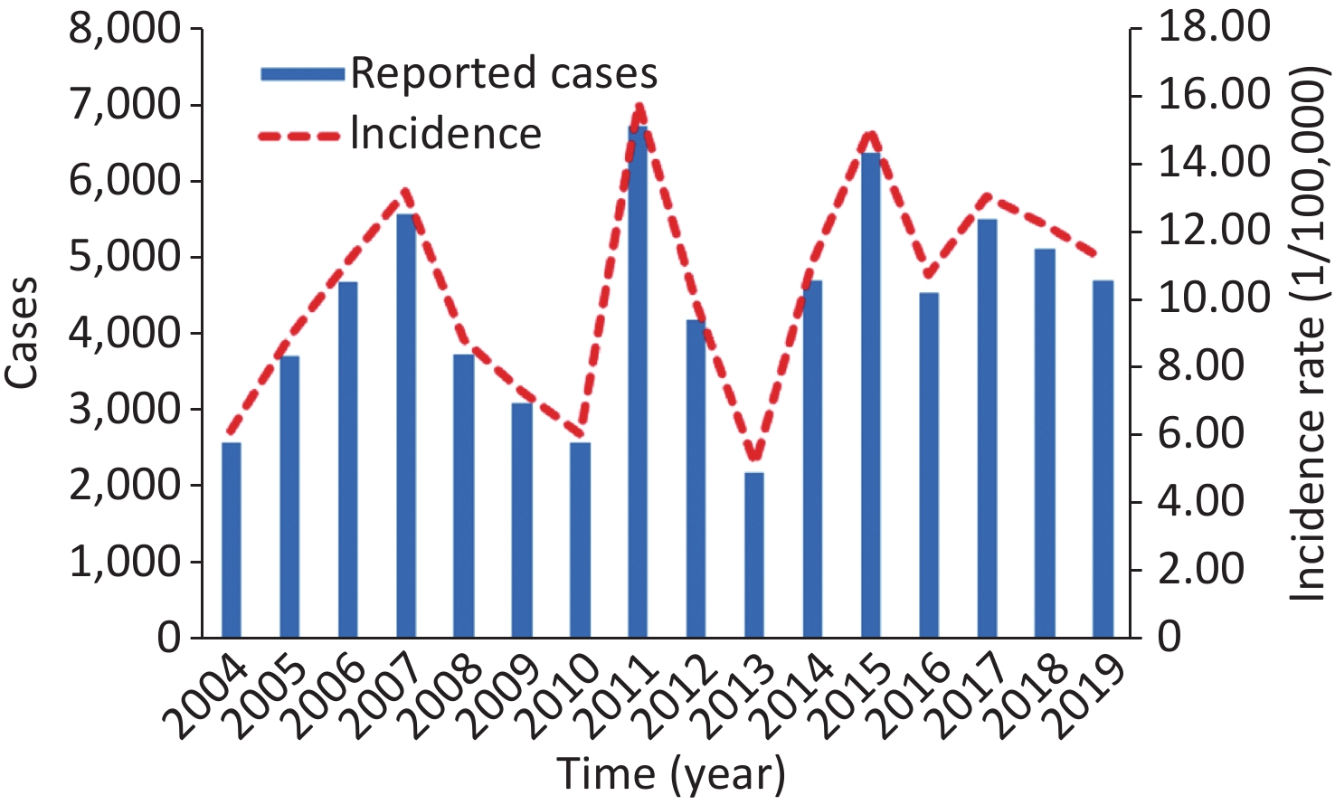
The study included a total of 70,020 incident cases in Liaoning during 2004–2019, showing an overall increase, but no statistical significance in SF morbidity was observed, with AAPC = 4.493 (95% CI: −22.278 to 40.485; t = 0.291, P = 0.771). The highest number of 6,728 cases (15.818 per 100,000 people) was recorded in 2011, which was 2.085 times higher than the lowest number of 2,181 cases (5.142 per 100,000 people) in 2013 (Supplementary Figure S1, available in www.besjournal.com). The decomposition results indicated that the number of SF epidemics relatively increased during 2004–2010 (average 9.256 per 100,000 people annually), with an AAPC of 6.758 (95% CI: −13.399 to 31.607; t = 0.613, P = 0.54) (Supplementary Figure S2, available in www.besjournal.com). However, an unexpected escalation was noted in 2011, and since then, it has remained relatively steady (average 11.024 per 100,000 people annually), with AAPC = 1.899 (95% CI: −12.966 to 19.302; t = 0.234, P = 0.815). SF morbidity was higher by a factor of 1.191 across the period 2004–2010 (IRR = 1.191, 95% CI: 1.188 to 1.193) (Supplementary Figures S1–S2). These results align with the SF resurgence in Hong Kong, China and South Korea^[8]. However, this trend did not align with the resurgence of SF in England^[2] in 2014. Moreover, the exact factors driving the increased pathogenicity of GAS are not fully understood. One probable explanation is the acquisition of novel prophages carrying new combinations of toxin and antimicrobial resistance genes. This is associated with the emergence and spread of predominant genotypes of emm12 and emm1 in China^[3]. Another explanation could be the natural cyclic patterns of the SF. As mentioned earlier, SF epidemics in China have exhibited an approximately six-year cycle^[9]. The unexpected surge since 2011 may indicate an emerging trend distinct from the previous phase of low morbidity. A third plausible reason is the relaxation of China’s two-child policy in 2011, which resulted in an increase in the number of susceptible populations. Fourth, improvements in the diagnostic capacity and increased awareness among medical workers may have contributed to the observed increase. Finally, worsening air quality in China may also be a contributing factor^[7].

Figure S1.  Yearly incident cases and incidence rate in Liaoning during 2004–2019. This plot pinpoints that the SF outbreak occurred in 2011 and there is a periodic cycle pattern of around 4–7 years.

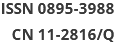
Figure S2.  A seasonal decomposition of the SF incidence series based on the STL technique. The (A) SF series is decomposed into (B) seasonal, (C) trend, and (D) irregular parts. It seems that there is a periodic outbreak pattern and a clear seasonality in SF incidence.

Remarkable semi-annual seasonality was observed in this study, with one peak in May–June and another in November–December (Supplementary Figure S3, available in www.besjournal.com). Different climatic features and the beginning of spring and autumn semesters might drive these peak activities^[2,7]. Our seasonal profile concurs with the prior literature in Hong Kong, China, South Korea^[8], and China′s mainland^[7]. However, it disagrees with earlier findings in England (peaking in February–March)^[2] and Poland (peaking in January–March)^[10]. This disagreement might be attributed to differences in school breaks, population density, socioeconomic status, lifestyle, climatic and ecological features, and predominant GAS emm gene types^[1,2,7]. In East Asia (including China), emm1 and emm12 are the predominant gene types responsible for SF outbreaks^[3], whereas in England, emm3, emm4, and emm12 are more prevalent^[2]. These variations in gene types may contribute to differences in the timing of SF peaks between East Asia and Europe^[3]. Additionally, SF epidemics remain at a low level in February each year, and some activities, such as the winter holidays and Spring Festival in China, could explain the reduced SF epidemics^[7].

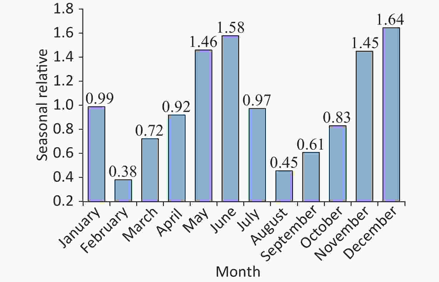
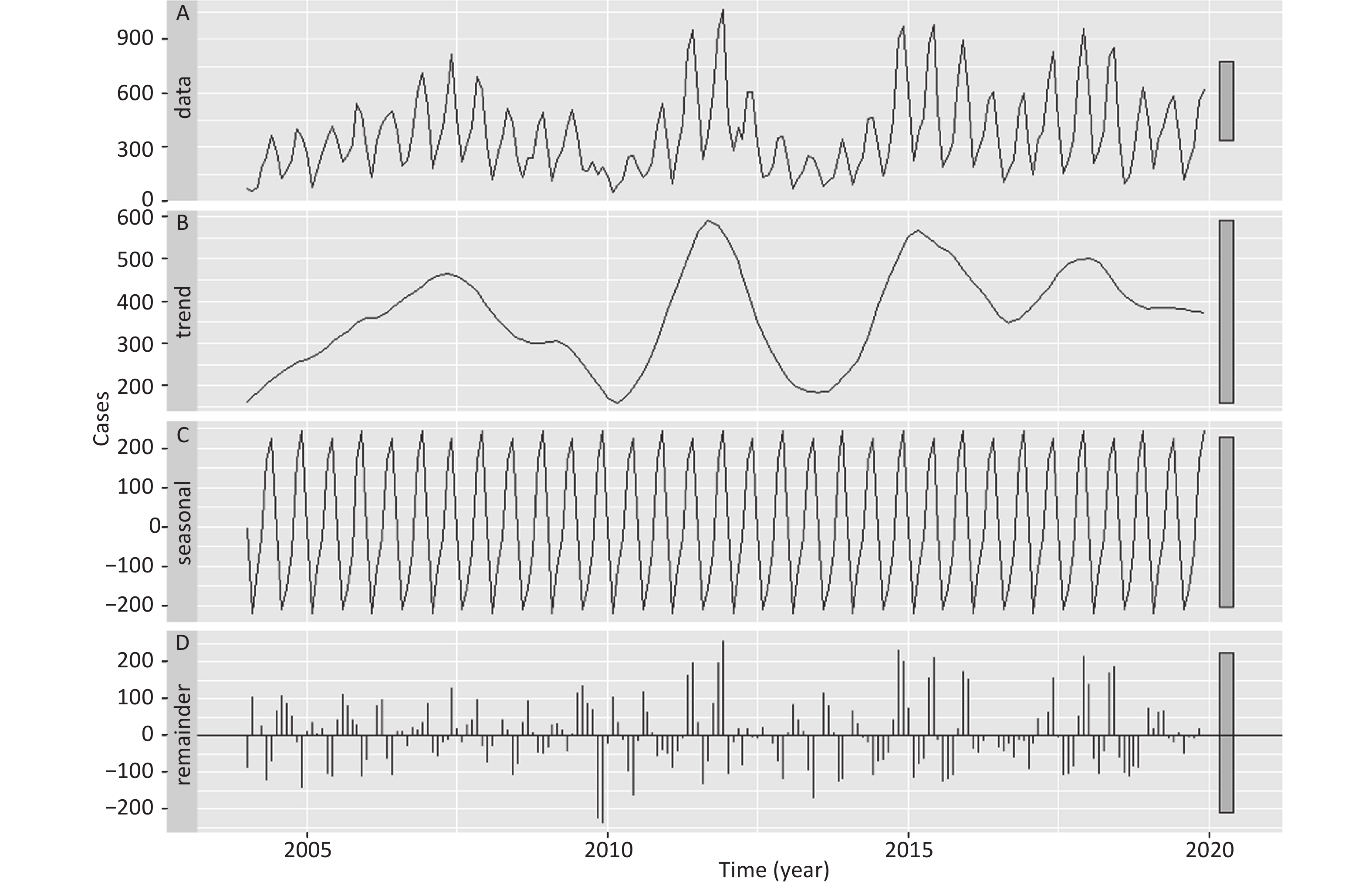
Figure S3.  The decomposed seasonal relative (SR) for the SF morbidity series using the multiplicative decomposition method. A value of SR = 1 means that the incidence for that period is exactly the same as the average. A value of SR > 1 means the incidence is higher than the average (indicating a high-risk season), and a value of SR < 1 means this period’s incidence is lower than the average (indicating a low-risk season). As shown, SF epidemics present pronounced dual seasonal patterns per year.

The SARFIMA parameters (including p, q, P, and Q) were estimated, and the number of differencing orders and preferred modes were selected by eliminating those with a lower log-likelihood (refer to Supplementary Materials [SARFIMA method], available in www.besjournal.com). Supplementary Table S1 (available in www.besjournal.com) summarizes the modes of the best SARFIMA (3, 0, 1)(3, −0.347, 0)₁₂, suggesting that the preferred model was selected as the one with mode 1. This model reported the maximum log-likelihood (−1193.7), coupled with the minimum Akaike’s information criterion (2411.391) and Bayesian information criterion (2449.706). Also, the autocorrelation function (ACF) and partial ACF results for the forecast error are provided in Supplementary Figure S4 (available in www.besjournal.com), showing most correlations were within the 95% CI. The Ljung-Box Q test ($ {\chi ^2} $ = 0.158, P = 0.691) indicated no serial correlations in the residuals. These checks confirmed a white noise series of forecast errors. Similarly, based on the modeling processes, SARFIMA (2, −0.302, 1)(1, 0.471, 2)₁₂ was selected as the optimal model fitted to the SF incidence series during 2004–2017; the model diagnoses for their key parameters and residuals are illustrated in Supplementary Table S2 and Supplementary Figure S5 (available in www.besjournal.com). Accordingly, a prediction of the future 12 and 24 data points was achieved based on these two best SARFIMA models (Table 1 and Supplementary Table S3, available in www.besjournal.com).

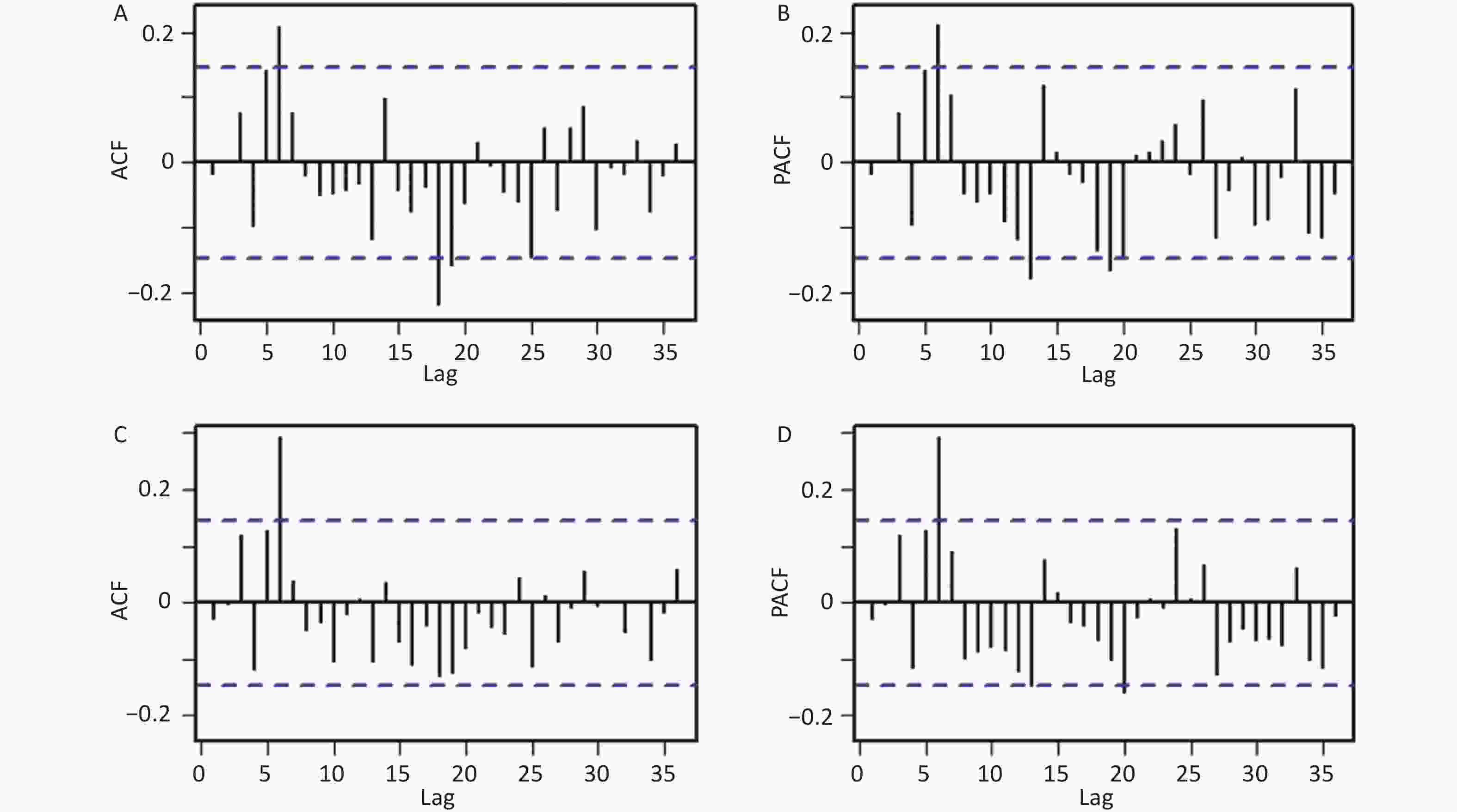
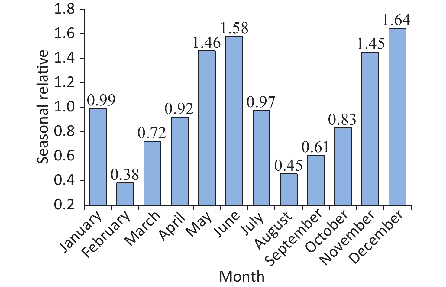
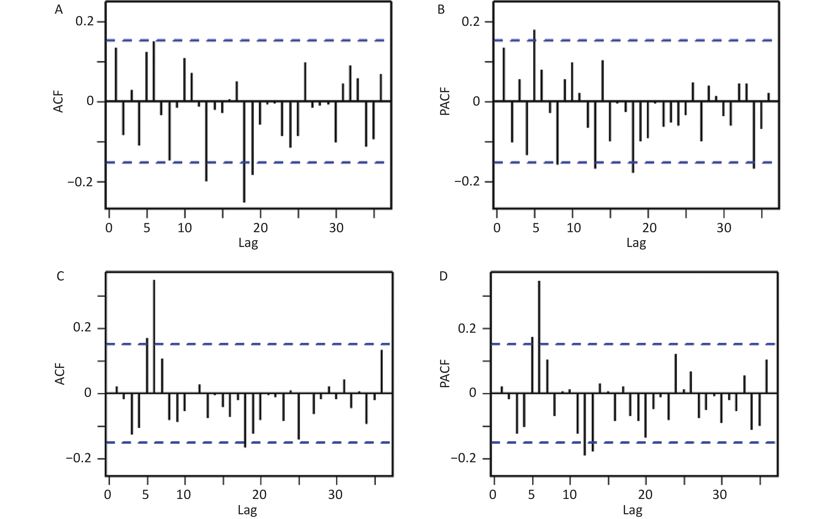
Figure S4.  ACF and PACF plots for the residual series under the SARIMA and SARFIMA. (A) ACF and (B) PACF plots for the residual series under the SARIMA, (C) ACF and (D) PACF plots for the residual series under the SARFIMA. Here the correlogram demonstrates that most spikes fall within the 95% CI except for few outside this significance bounds (which is also reasonable because some high-order correlations easily exceed the significance bounds by chance alone), indicating that there is little evidence of non-white noise in the forecast errors.

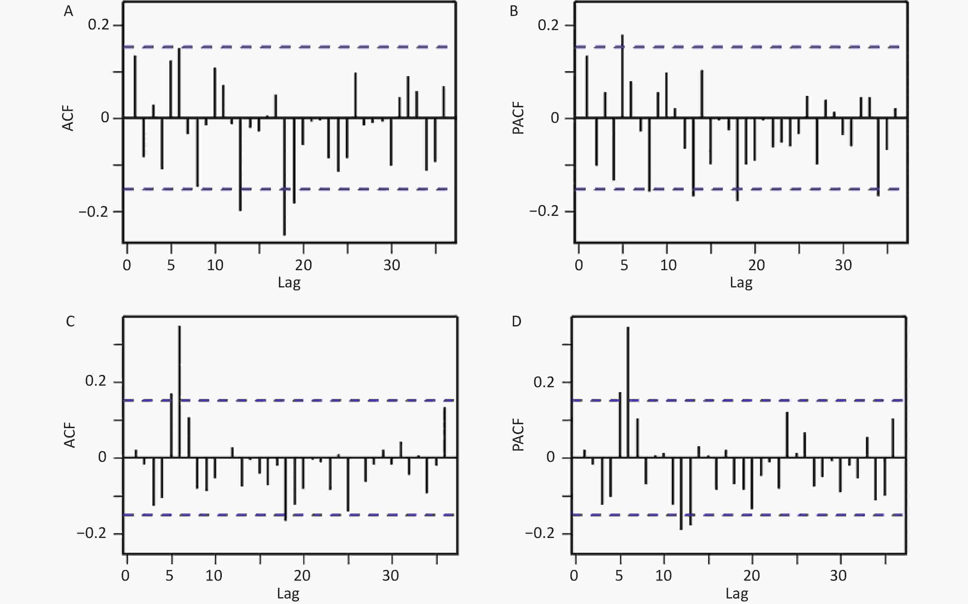
Figure S5.  ACF and PACF plots for the residual series under the SARIMA and SARFIMA based on the data during 2004-2017 in Liaoning. (A) ACF and (B) PACF plots for the residual series under the SARIMA, (C) ACF and (D) PACF plots for the residual series under the SARFIMA. Here the correlogram demonstrates that most spikes fall within the 95% CI except for few outside this significance bounds (which is also reasonable because some high-order correlations easily exceed the significance bounds by chance alone), indicating that there is little evidence of non-white noise in the forecast errors.

Additionally, we identified the SARIMA (3, 0, 1)(3, 1, 0)₁₂ and SARIMA (2, 1, 2)(1, 1, 2)₁₂ specifications based on the modeling steps as the best models for the incidence series during 2004–2018 and 2004–2017, respectively (refer to Supplementary Materials [SARIMA method], Supplementary Table S4, and Supplementary Figure S6, available in www.besjournal.com). Further diagnostic checks for residuals are provided in Supplementary Figures S4–S5 and Supplementary Table S4. Figure 1 and Table 2 compare the forecasting accuracy and reliability of SARIMA and SARFIMA. The MAD, MAPE, RMSE, RMSPE, and MER values under SARFIMA were lower than those under SARIMA for these two datasets. This indicates that SARFIMA offered a clearer perspective than SARIMA on capturing the dynamic dependency structure in the spread of SF. Previous literature has also indicated that SARFIMA is sufficient for forecasting oil supply, road fatality rate, temperature, and hemorrhagic fever with renal syndrome, and some generate more accurate results than SARIMA^[6]. These studies provide additional support for our findings and reinforce the usefulness of SARFIMA as a promising alternative for analyzing SF trends and seasonality.

Figure 1.  Comparison of the observed curves with the forecast curves under the SARIMA and SARFIMA. (A) 12 hold-out data forecasts under the SARIMA in Liaoning, (B) 12 hold-out data forecasts under the SARIMA in mainland China, (C) 12 hold-out data forecasts under the SARFIMA in Liaoning, and (D) 12 hold-out data forecasts under the SARFIMA in mainland China. The grey shaded area signifies the forecasted curve with 95% CI in plots. It appears that the forecasts under the SARFIMA are closer to the observed curves.

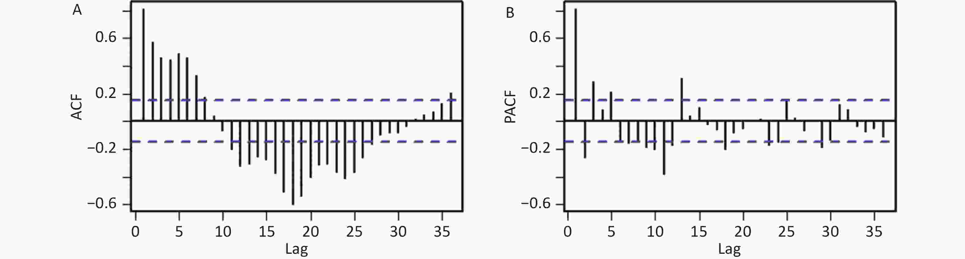
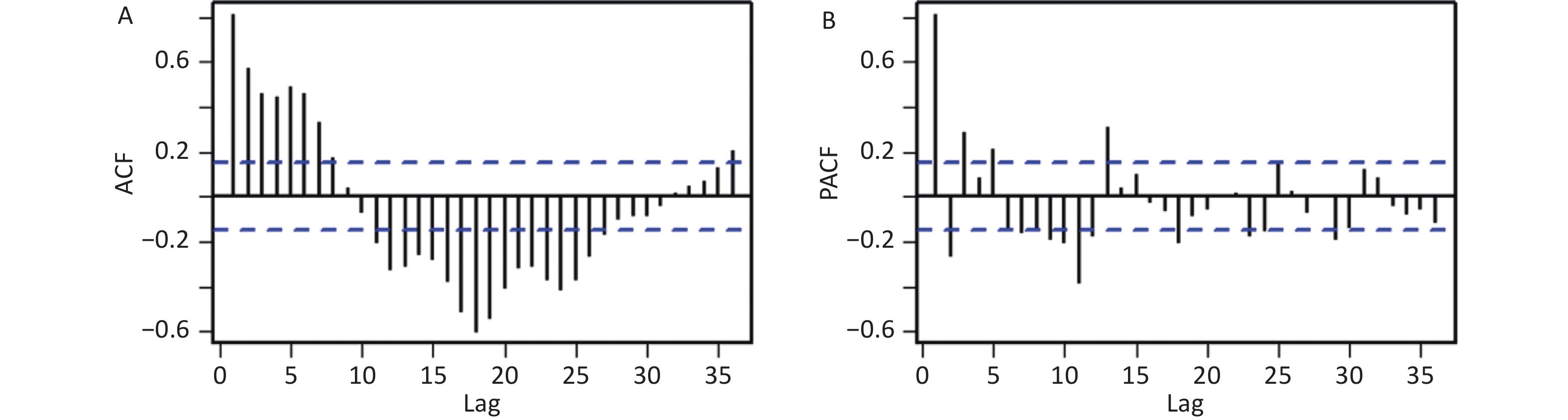
Figure S6.  ACF and PACF plots for the seasonally differenced series in Liaoning. (A) ACF plot, and (B) PACF plot. The significant spike at lag 3 in the PACF indicates that the maximum orders may be 3 in the non-seasonal AR component, the significant spike at lag 10, 11, and 12, along with 23, 24, and 25 in the ACF suggests that the maximum orders may be 3 in the seasonal AR component. The significant spikes at lag 12, 24, and 36 in the ACF suggests that the maximum orders may be 1 in the seasonal MA component.

SARFIMA extends SARIMA, replacing the differencing term with fractional integration. With the introduction of fractional integration^[6], SARFIMA has the potential to capture long-range dependence and long memory effects in SF incidence series; it enables better capture of nonlinear patterns and complexities; it can offer more flexibility in modeling the dependence structure of SF epidemics; it can accommodate both seasonal and non-seasonal series, allowing for the modeling of multiple seasonal patterns; and it becomes robust to outliers because the inclusion of long memory helps to smooth out the effects of outliers. This explains why SARFIMA generates more accurate and flexible predictions than SARIMA. Considering the appeal of SARFIMA, the importance of this sophisticated model as a powerful forecasting tool should be underscored when analyzing the temporal levels of other communicable diseases. However, further validation is required to confirm this finding. Furthermore, several new advanced statistical techniques, such as Bayesian structural time series, flexible transmitter networks, error-trend-seasonal frameworks, and age-structure mathematical models, have recently emerged, showing potential for time series forecasting. Consequently, studies that specifically focus on comparing the predictive quality of SARFIMA with the aforementioned techniques are essential.

This study has several limitations. First, because SF has become a milder disease with a low fatality rate since the 20th century^[10], patients with mild symptoms may not seek medical attention, leading to underreporting and underdiagnosis of SF cases. Second, owing to the unavailability of data from to 2020–2023, we only used data from 2004–2019 to indicate model performance. The COVID-19 outbreak significantly changed the SF epidemic trend from 2020–2023. Thus, the model should be regularly updated by incorporating new data to ensure reliable forecasting. Third, the findings of this study pertain specifically to how well SARFIMA estimates SF epidemics. Additional studies are needed to validate the efficiency of this method in estimating epidemics of other communicable diseases. Fourth, 100 or more observations are anticipated to be used to construct SARFIMA in applications. Finally, although SARFIMA with exogenous variables could potentially offer a higher forecasting accuracy, we could not obtain these SF-related variables; hence, further analyses were excluded.

In summary, SARFIMA is a versatile model that can capture both short- and long-term dependencies in SF incidence as well as seasonal patterns. Its ability to capture complex dynamics and accurately forecast SF epidemics enables it to have advantages over SARIMA. Consequently, SARFIMA should be considered a valuable alternative for estimating SF epidemics to make informed decisions, optimize resources, and plan for the future. Furthermore, the incidence of SF remains high in Liaoning under current interventions. This highlights the need for additional preventive and control measures to address this evolving situation.