


-
Scarlet fever (SF) is a common communicable disease that results from group A Streptococcus (GAS) infections[1]. SF accounted for the global loss of life among children 5–15 years of age in the 18th and 19th centuries[2]. A rapid reduction in SF morbidity and mortality occurred due to the scale-up of effective antibiotics and improvements in sanitation and nutrition[3]. The unexpected increase in the incidence of SF has attracted a renewed interest in infectious diseases[3]. Because the triggers that cause SF outbreaks are not fully understood and there is a scarcity of available vaccines protecting susceptible populations from GAS infections, effective prevention and control plans are required to stop the continued spread of SF.
Time series analysis assists in the development of hypotheses to explain the temporal patterns of different diseases and to analyze the spread, therefore, facilitating the creation of a quality forecasting system. The seasonal autoregressive integrated moving average (SARIMA) model has been widely applied to estimate the epidemiological patterns of contagious diseases because this model has a simple structure, fast applicability, and a relatively high forecasting reliability level [4]. It has been shown that the SARIMA model is able to satisfactorily estimate a simple time series [4], but it is difficult to manage complex time series, such as the data with multiple seasonal periods, high-frequency seasonality, non-integer seasonality, and dual-calendar effects. By comparison, the innovation state-space modelling framework that combines Box-Cox transformations, Fourier series with time-varying coefficients, and autoregressive moving average (ARMA) error correction (known as the TBATS method) is customized for use with the patterns included in a complex time series described above [5]. In addition, the TBATS model is used for linearity and some types of non-linearity in a complex time series based on Box-Cox transformations [5], which makes it possible to perform a multistep ahead prediction. Moreover, the TBATS model is able to decompose a complex seasonal time series into its trend, seasonal, and irregular components [5], which is not able to be undertaken by use of the SARIMA model. Importantly, SF morbidity has been shown to display dual seasonal patterns in some countries. Therefore, this study analyzed the long-term epidemic patterns using the TBATS model. The forecasting power under the TBATS model was compared with the SARIMA model.
We obtained the monthly SF incidence and population data between January 2004 and December 2019 from the Chinese CDC and the Statistical Yearbook of China, respectively. Then, we partitioned the SF morbidity series into two segments comprising a training dataset from January 2004 to December 2017 to construct the SARIMA and TBATS models and a testing dataset from January 2018 to December 2019 to test the generalization of both models. Two additional datasets were provided to test the robustness of both models: the first 180 data sets from January 2004 to December 2018 and 156 data sets from January 2004 to December 2016 were treated as training datasets, respectively; and the remainder were testing datasets. We estimated the changing epidemiologic trends of SF based on annual percentage change (APC) and average APC (AAPC) using the Joinpoint regression program (version 4.8.0.1). We constructed the TBATS model with the “forecast,” “tseries,”, and “FinTS” packages in R software (version 3.4.3). The incidence rate ratio (IRR) with a 95% uncertainty limit (UL) before and after the SF outbreak was calculated using the method proposed by Armitage and Berry [6]. The mean absolute deviation (MAD), root mean square error (RMSE), mean absolute percentage error (MAPE), mean error rate (MER), and root mean square percentage error (RMSPE) were computed to compare the forecasting ability of both models.
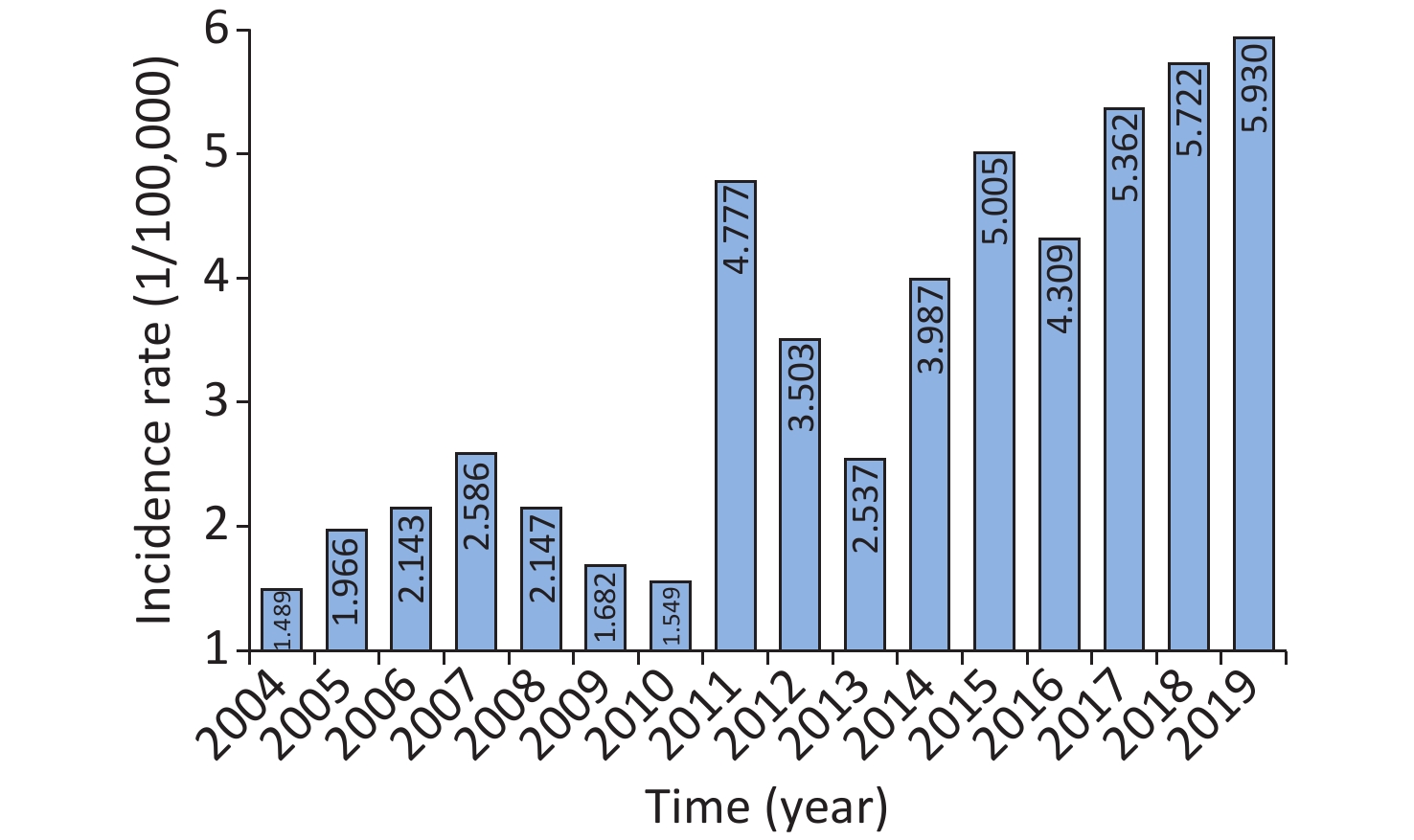
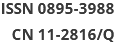
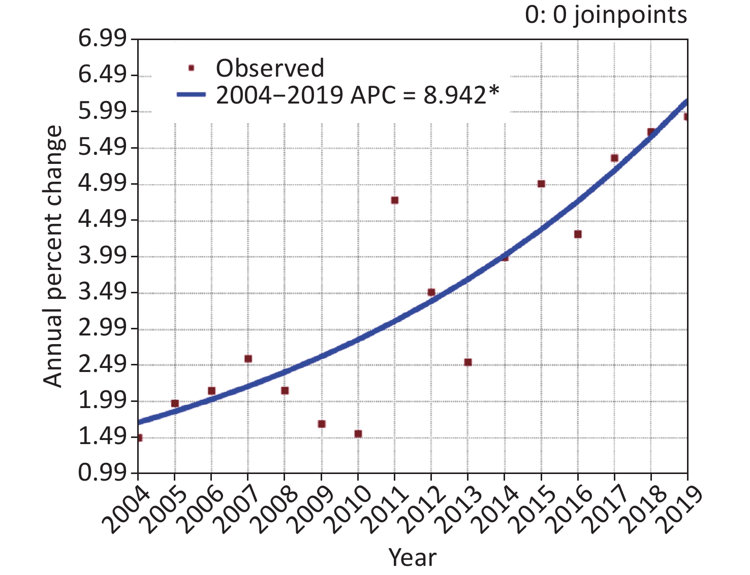
During the study period, a notable increase in SF morbidity was detected, with an AAPC = 8.942 (95% UL: 5.995–11.971; t = 6.697, P < 0.001; Supplementary Figure S1, available in www.besjournal.com), and the highest morbidity (5.930/100,000 persons) occurred in 2019, which increased by a factor of nearly four compared with the lowest level (1.489/100,000 population) in 2004 (Supplementary Figure S2, available in www.besjournal.com). The SF epidemics remained relatively steady from 2004–2010 (average, 1.937/100,000 persons annually), with an AAPC = −0.840 (95% UL: −7.678 to 6.505; t = −0.231, P = 0.817). An unexpected outbreak was witnessed in 2011, and since then a rapidly increasing trend occurred (average, 4.580/100,000 persons annually [excluding 2013]; the exact causes regarding this annual drop are unknown; Supplementary Figure S2), with an AAPC = 5.952 (95% UL: 0.239–11.992; t = 2.466, P = 0.043), which showed good agreement with a resurgence of SF in Hong Kong, China[7], but inconsistent with England where the resurgence occurred in 2014 [8]. There has been a doubling in the SF incidence during the post-resurgence periods compared with the pre-resurgence periods (IRR = 2.364, 95% UL: 2.358–2.370). Nevertheless, the driving force associated with the increased pathogenicity of GAS fails to be elucidated. A possible explanation may be due to the acquisition of novel prophages harboring new hybridizations of toxin genes and antimicrobial resistance genes, which is related to the emergence and expansion of the predominant genotypes of emm12 and emm1 in China [3]. Another explanation may be associated with the natural periodicity of the SF incidence (SF epidemics are characterized by a cyclic change of approximately 6 years [3]). A third explanation may be linked to the relaxation of the 2-child policy in 2011 [3], which led to an increase in the number of susceptible individuals. A fourth reason may be attributed to improvements in the diagnostic capacity and the increased awareness of medical workers in reporting SF [3]. A fifth reason may be a result of the deterioration of air quality in China [9], despite the gradual improvements in the last 2 years. Finally, there are no vaccines available to prevent infections with GAS until now.
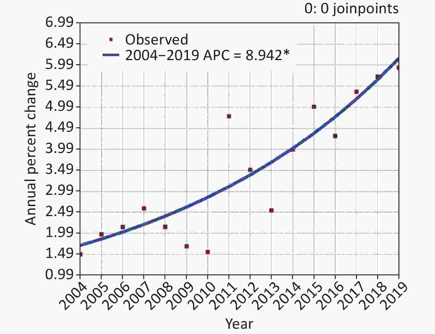
Figure S1. Joinpoint regression showing the scarlet fever epidemic trends in the period 2004–2019. *Showed that the annual percent change (APC) is significantly different from zero at the significance level. This plot was plotted using Joinpoint regression program (Version 4.8.0.1). Joinpoint is a statistical tool for the description and analysis of trends with the Joinpoint methods. This Joinpoint Regression Program is designed as a Windows-based statistical software package to analyze Joinpoint methods. Users can use this software to investigate whether there is a statistically notable change in trend (Available from https://surveillance.cancer.gov/joinpoint/. Accessed on 16 May 2022).
Figure S2. The yearly incidence of SF from 2004 to 2019. It was seen that SF had the lowest incidence in 2004 (1.489 per 100,000 population) and the highest morbidity in 2019 (5.930 per 100,000 persons).
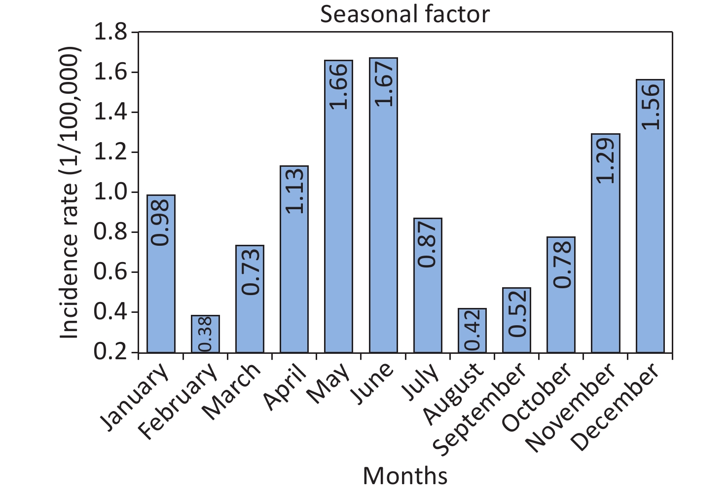
A marked semi-annual seasonal behavior occurred in the monthly SF incidence, with a strong peak between May and June, and a weak peak between November and December (Supplementary Figures S3–S4, available in www.besjournal.com). We surmised that different climatic features and beginning of spring and autumn semesters contributed to this difference in the margin of peak activities. Our seasonal profile correlates well with previous findings from Hong Kong, China [7]; however, discordant with that in England, which peaked between February and March [8]. This inconsistency may be due to the different school breaks, population density, and different GAS emm gene types in east Asia and Europe [1, 8]. In addition, the SF epidemics retain the lowest level in February every year (Supplementary Figure S3), attributable to the winter holidays and the Spring Festival.
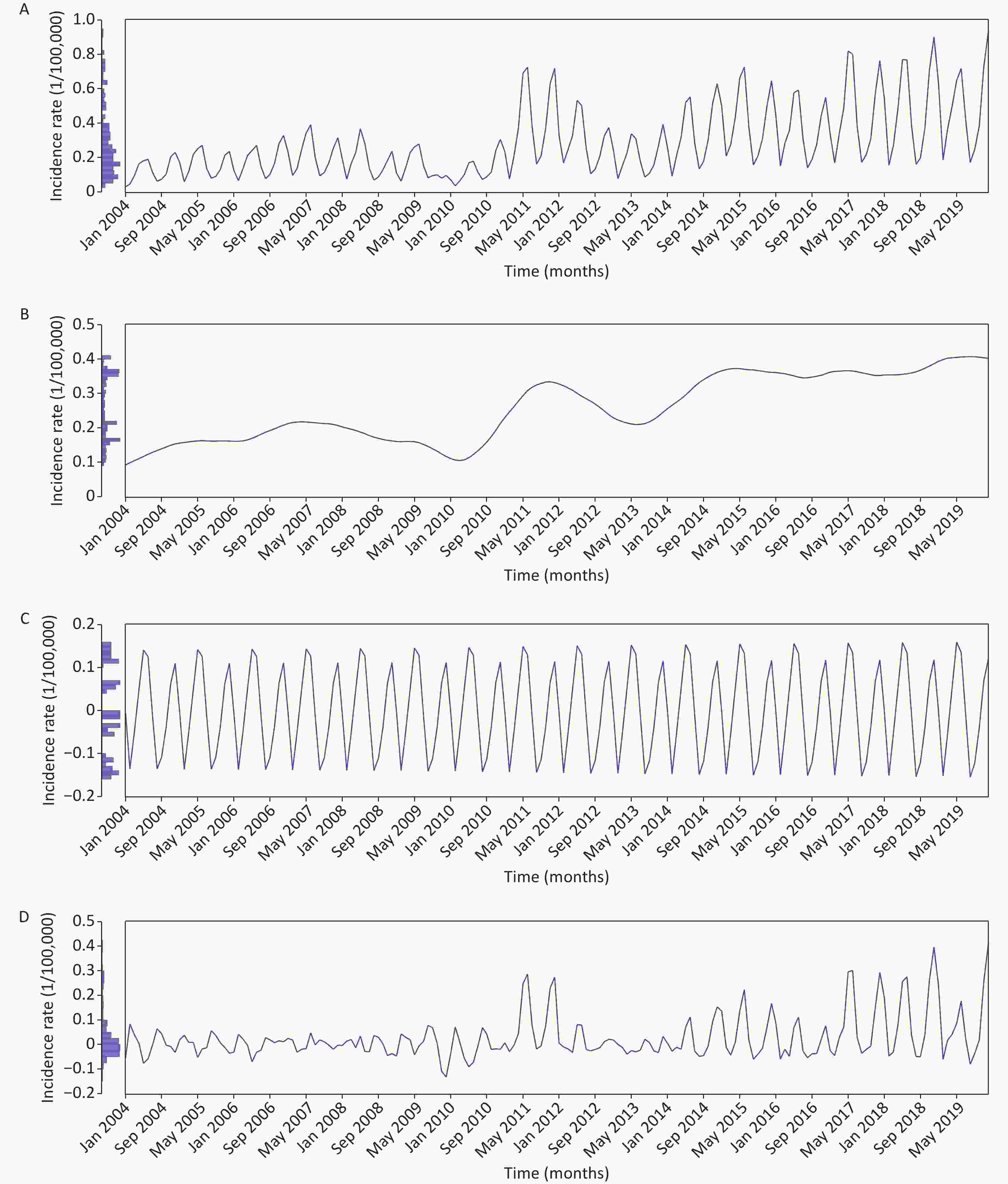
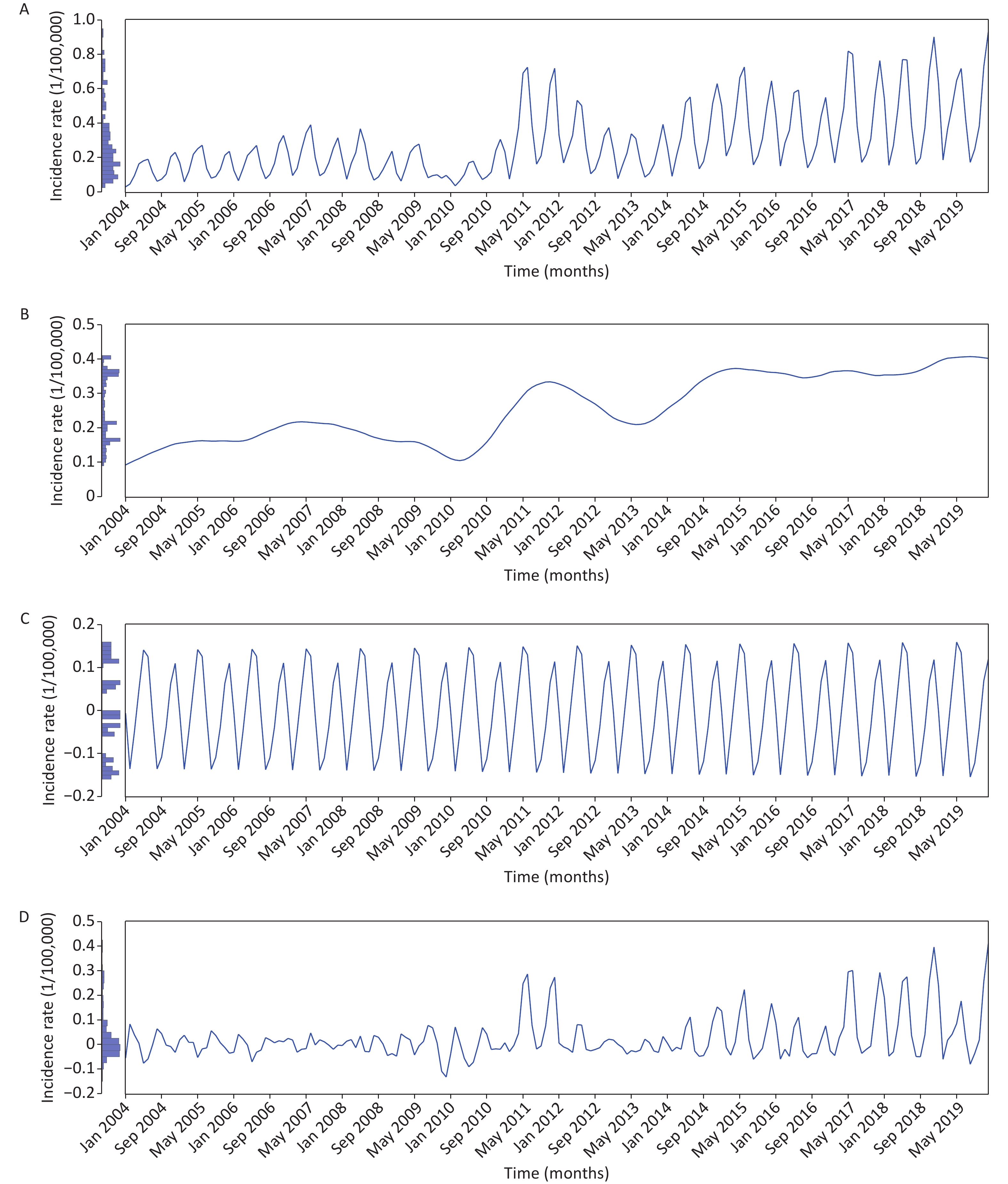
Figure S3. Time series plot showing the monthly SF incidence rate and the decomposed seasonal, trend, and irregular components based on the STL technique. (A) Original monthly SF morbidity series. (B) Decomposed trend component. (C) Decomposed seasonal component. (D) Decomposed random component. As illustrated, overall the SF morbidity showed a rising tendency, with a sudden increase in 2011, and having notable seasonal patterns.
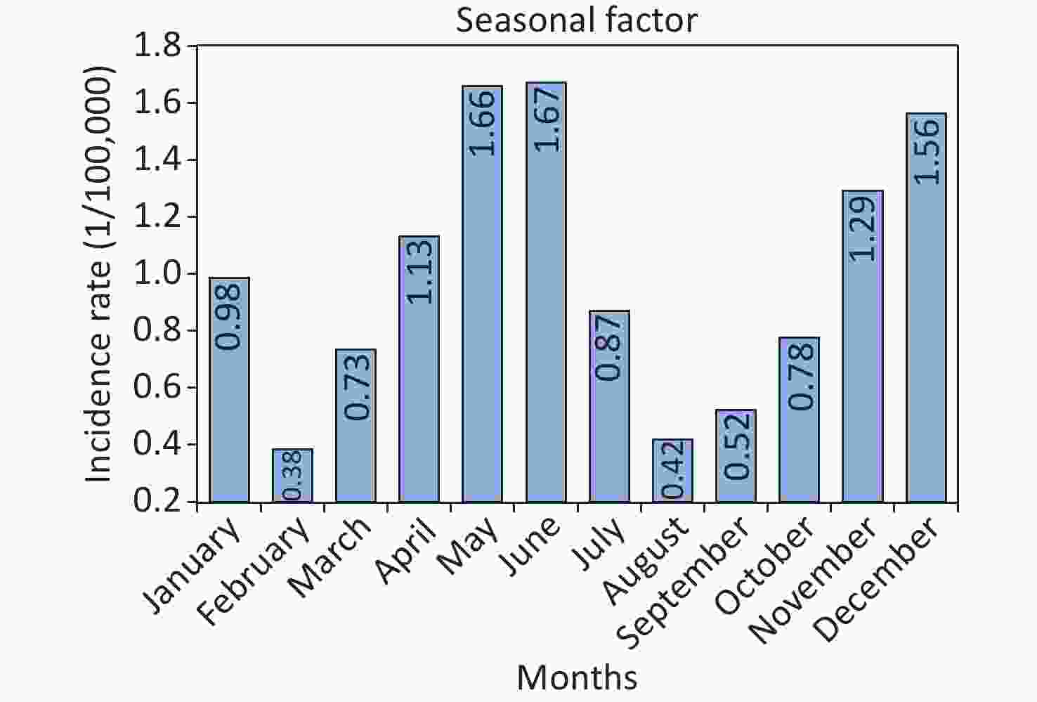
Figure S4. The decomposed seasonal factors for the scarlet fever morbidity series using the multiplicative decomposition method (The classical Seasonal Decomposition technique can be applied to decompose a time series into a seasonal pattern, a trend component, and a random fluctuation component. This technique is implemented based on the ratio-to-moving-average method. The Seasonal Decomposition technique can be divided into two types including a multiplicative and an additive method. For a multiplicative decomposition method, the seasonal component is a factor by which the seasonally adjusted series is multiplied to produce original observed values. For a time series without seasonal variation, the seasonal pattern is deemed as one. For an additive decomposition method, the seasonal adjustments are added to the seasonally adjusted series to yield the original series. For the morbidity series of infectious diseases, the multiplicative decomposition method typically produces a more reliable decomposed result in application. By employing a multiplicative decomposition method to an object series, the seasonal pattern or seasonal factors included in the object series can be obtained. Such a decomposition is very helpful in removing the seasonal effect from a series so that we can visibly look into the other characteristics of interest in the series that may be masked by the seasonal trait[7,8]).
The forecasts under the TBATS approach rely largely on the number of harmonics ki applied for each seasonal pattern. As a result, in selecting the number of harmonics ki, considering one seasonal component each time, we then fitted the model on the target data repeatedly via gradually increasing the number of harmonics ki, but holding the remaining harmonics constant for each i until the optimal AIC is obtained. In determining the most suitable orders (p and q) of the ARMA model, we used the automatic procedure proposed by Hyndman and colleagues[10] to fit the forecasting residuals. If the selected model with the ARMA (p, q) residual component generates a smaller AIC than the one model without the ARMA (p, q) residual component, this selected specification would be considered as the best possible model; otherwise, the ARMA (p, q) residual component is deleted. After modelling by trial and error, the TBATS (0.04, {4,0}, 0.882, {<12,5>}) specification was selected as the optimal model in that the minimum AIC (−197.965) was detected in this model, and the identified key parameters of this best TBATS model are reported in Supplementary Table S1, available in www.besjournal.com. Additional statistical diagnoses for the forecast errors are provided in Supplementary Table S2 and Supplementary Figures S5–S6, available in www.besjournal.com. The Ljung-Box Q statistics of the forecast errors produced a Q(18) = 11.442 with a P-value of 0.875, indicating no serial correlations in this residual series. Moreover, the ARCH effect was largely removed because the LM(18) = 23.808 with a P-value of 0.302. These results confirmed the adequacy of the model specifications. Similarly, based on the modelling steps described above, the TBATS (0.01, {0,0}, 0.898, {<12,5>}) and TBATS (0.048, {0,0}, 0.902, {<12,5>}) specifications tended to be the preferred models for forecasting the 12- and 36-holdout periods (Supplementary Tables S3–S4 and Supplementary Figures S7–S10, available in www.besjournal.com).
Parameters 24-step ahead forecasting 12-step ahead forecasting 36-step ahead forecasting TBATS (0.04, {4,0}, 0.882,
{<12,5>}) modelTBATS (0.01, {0,0}, 0.898,
{<12,5>}) modelTBATS (0.048, {0,0}, 0.902,
{<12,5>}) modelLambda 0.0401 0.0105 0.0480 Alpha 0.1652 0.6489 0.6795 Beta −0.0252 −0.0362 −0.0432 Damping Parameter 0.8818 0.8982 0.9024 Gamma-1 Values 0.0002 −0.0046 −0.0048 Gamma-2 Values −1.2682 0.0050 0.0072 AR coefficients AR1 = 0.4772, AR2 = 0.2318,
AR3 = −0.1894, AR4 = 0.3222− − Seed states 1 −2.3530 −2.4373 −2.3215 2 0.1089 0.1130 0.1015 3 −0.0246 −0.0185 −0.0251 4 −0.0748 −0.0757 −0.0731 5 −0.0069 −0.0077 −0.0065 6 0.0213 0.0266 0.0207 7 0.0296 0.0312 0.0279 8 −0.1547 0.1489 0.1353 9 −0.5953 −0.6307 −0.5756 10 −0.0602 −0.0649 −0.0598 11 0.1463 −0.1521 −0.1404 12 −0.0231 −0.0248 −0.0218 13 0.0000 − − 14 0.0000 − − 15 0.0000 − − 16 0.0000 − − Sigma 0.1686 0.1909 0.1797 AIC −197.9650 −175.3322 −198.4532 Parameters 48-step ahead forecasting 72-step ahead forecasting Future 36-step ahead forecasting TBATS (0.037, {0,0}, 0.901,{<12,5>}) TBATS (0.029, {0,0}, 0.87,{<12,4>}) TBATS (0.023, {0,0}, 0.895, {<12,5>}) Lambda 0.0368 0.0292 0.0225 Alpha 0.6900 0.7253 0.6444 Beta −0.0410 −0.1128 −0.0378 Damping Parameter 0.9013 0.8702 0.8955 Gamma-1 Values −0.0069 −0.0115 −0.0050 Gamma-2 Values 0.0052 0.0035 0.0037 AR coefficients − − − Table S1. The best TBATS models obtained on the basis of different datasets and their key parameters
Lags SARIMA model TBATS model Box-Ljung Q P LM-test P Box-Ljung Q P LM-test P 1 0.044 0.833 0.001 0.979 0.005 0.943 52.651 < 0.001 3 1.944 0.584 2.364 0.500 0.235 0.972 22.234 < 0.001 6 3.720 0.715 4.223 0.647 1.246 0.975 23.555 0.001 9 6.093 0.731 5.981 0.742 4.538 0.873 23.624 0.005 12 13.021 0.368 9.427 0.666 7.320 0.836 23.416 0.024 15 13.094 0.595 12.379 0.650 10.456 0.790 23.533 0.073 18 13.663 0.751 19.872 0.340 11.442 0.875 24.550 0.138 21 17.313 0.692 20.262 0.505 19.031 0.583 23.808 0.302 24 23.237 0.506 29.352 0.207 23.061 0.516 24.015 0.461 27 26.060 0.515 25.492 0.547 23.466 0.660 23.924 0.635 30 26.082 0.671 26.422 0.653 25.230 0.714 24.918 0.729 33 29.133 0.660 29.863 0.624 29.004 0.667 24.941 0.842 36 41.417 0.246 37.230 0.412 30.707 0.718 24.391 0.929 Note. SARIMA seasonal autoregressive integrated moving average method, TBATS an advanced innovation state-space modelling framework by combining Box-Cox transformations, Fourier series with time-varying coefficients, and autoregressive moving average (ARMA) error correction. Table S2. Box-Ljung Q and LM tests for the residual series of the SARIMA and TBATS models
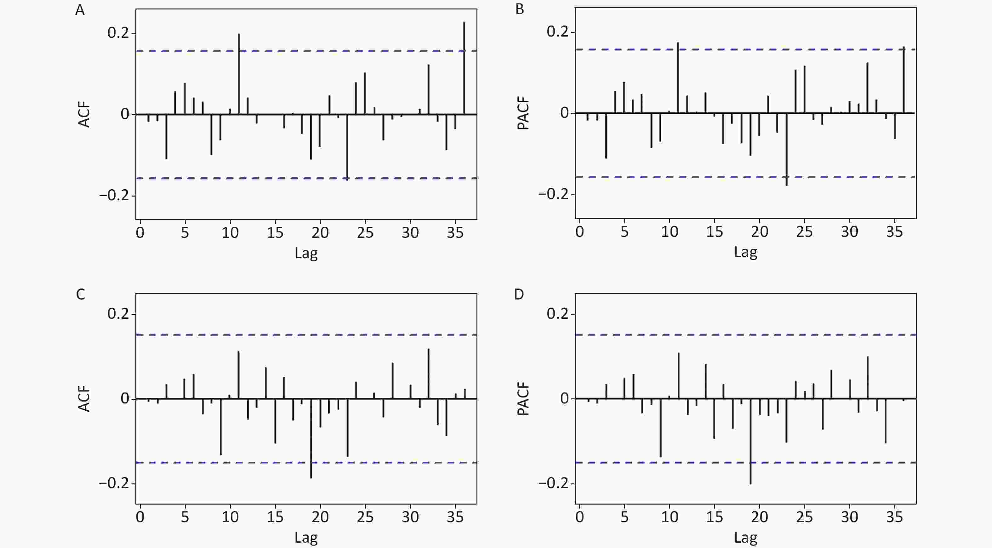
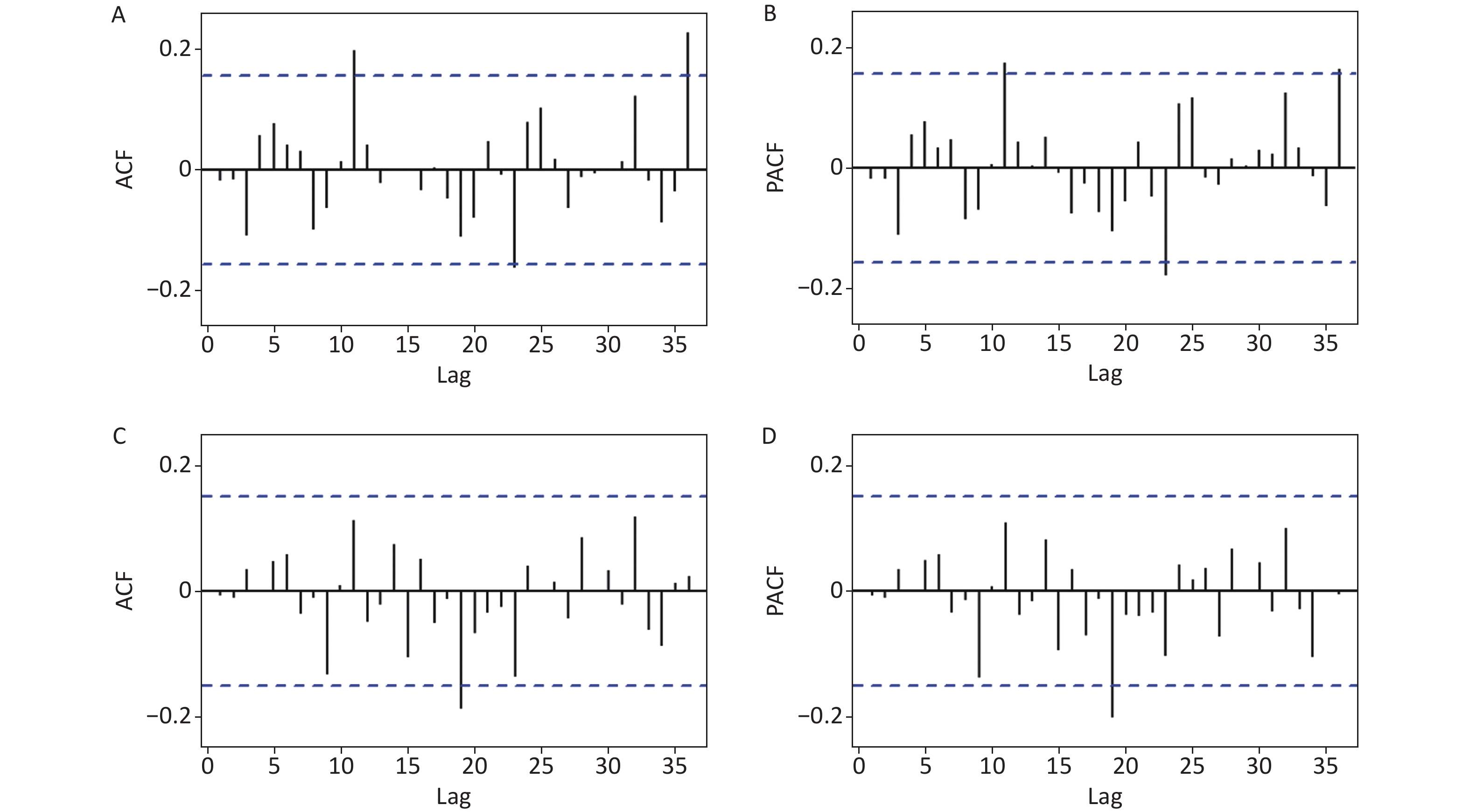
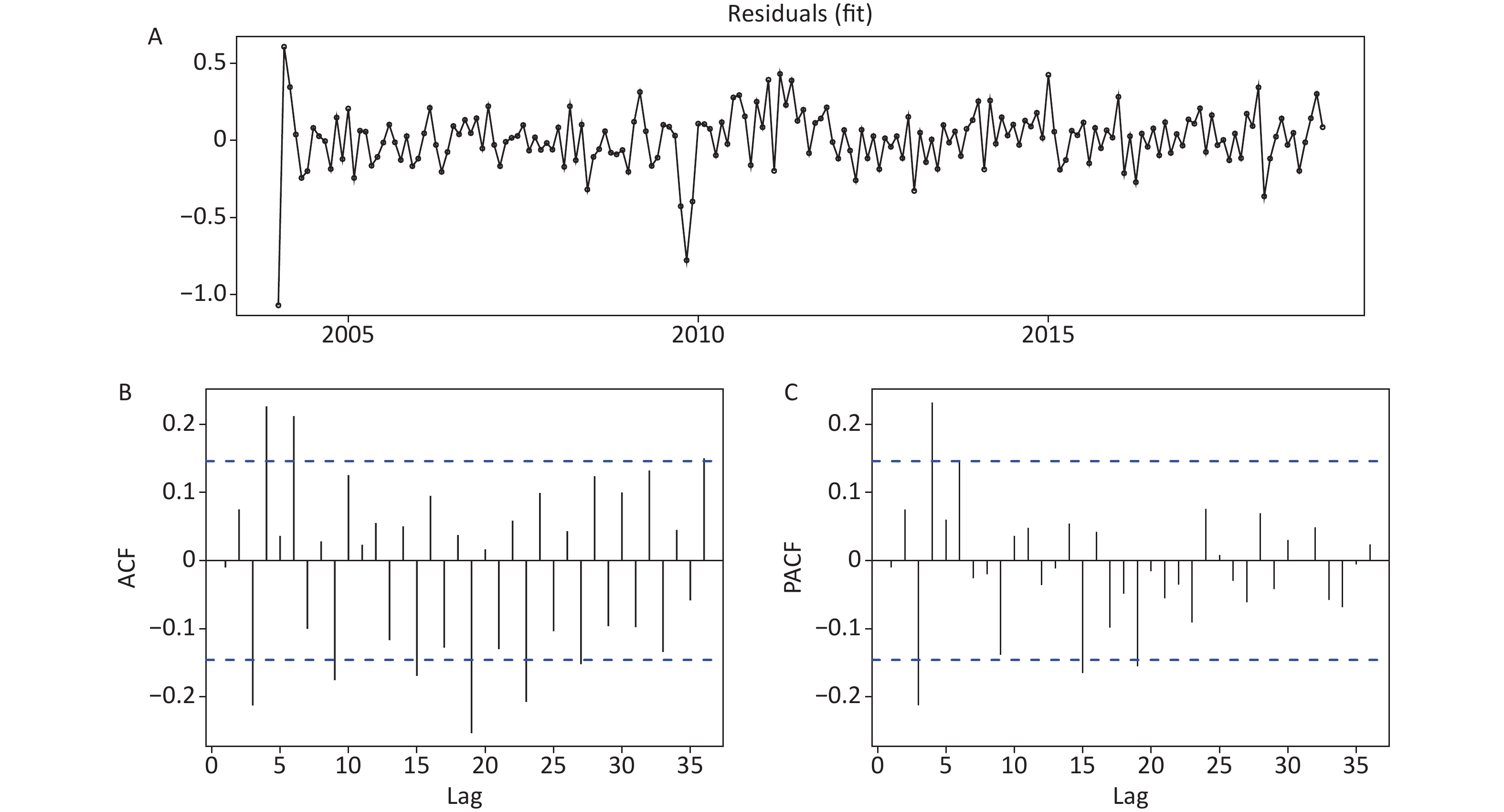
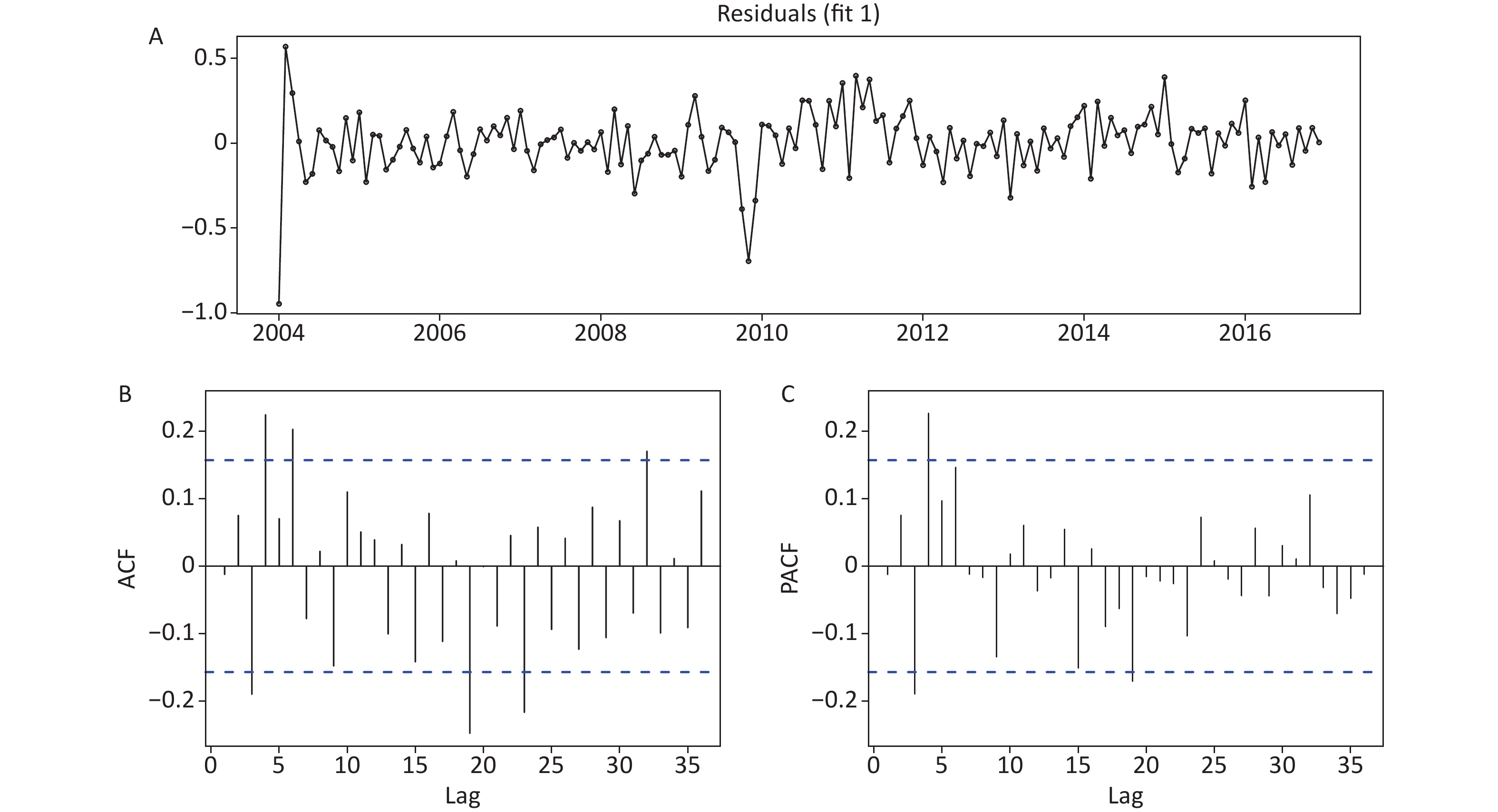
Figure S5. Estimated autocorrelation function (ACF) and partial ACF (PACF) plots to display the statistical checking for the residual series of the SARIMA and TBATS models. (A) ACF plot for the SARIMA model. (B) PACF plot for the SARIMA model. (C) ACF plot for the TBATS model. (D) PACF plot for the TBATS model. We can see that the correlation coefficients at lags 11, 23, and 36 in Figure 2A and 2B, and at lag 19 in Figure 2C and 2D touched the confidence levels (this is reasonable as the correlation coefficients at higher-order may exceed the significance bounds by chance alone), but all other correlation coefficients at different lags failed to touch the confidence levels, seemingly suggesting effective and sufficient models.
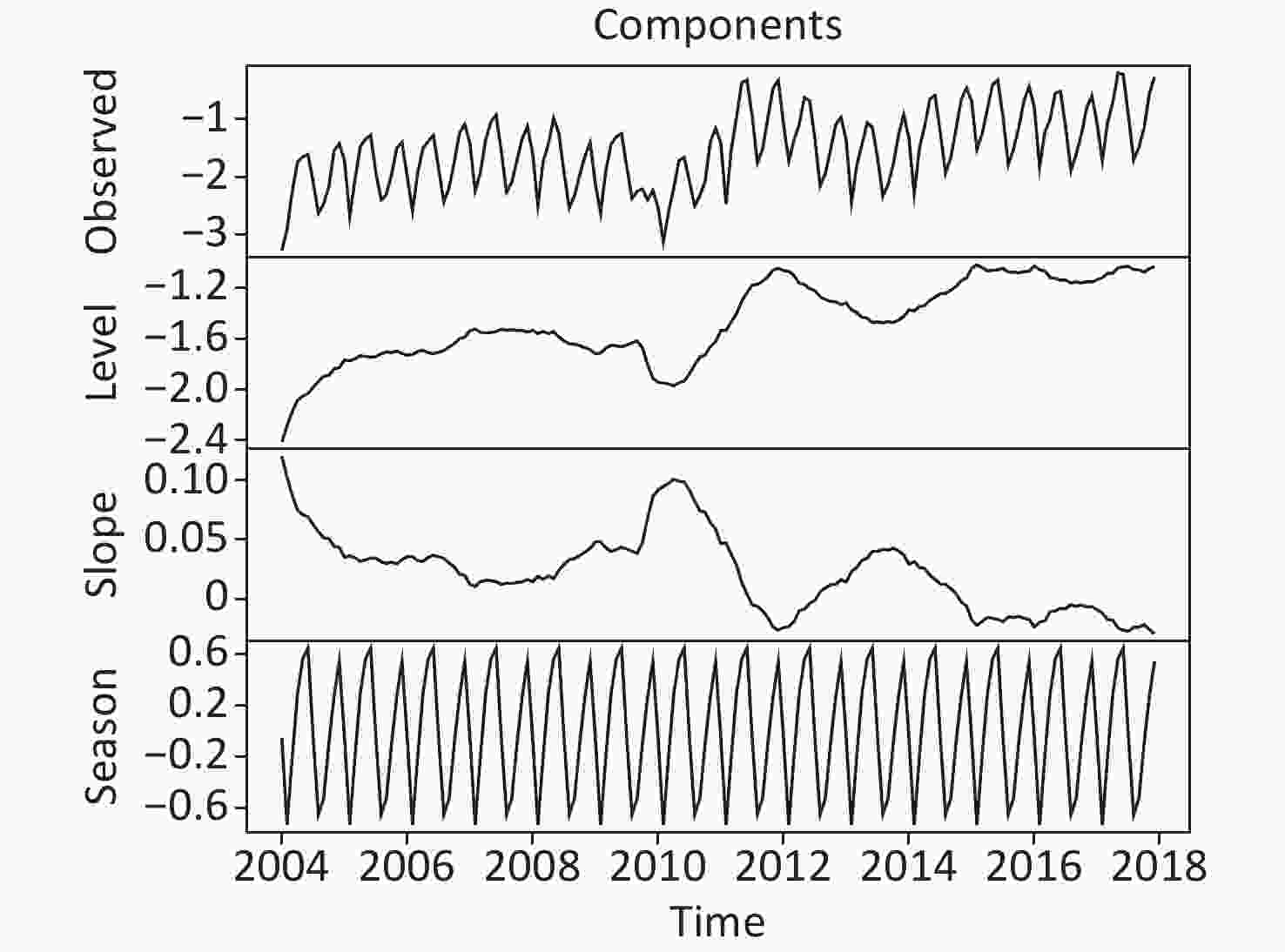
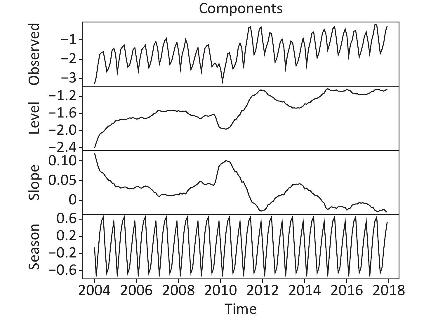
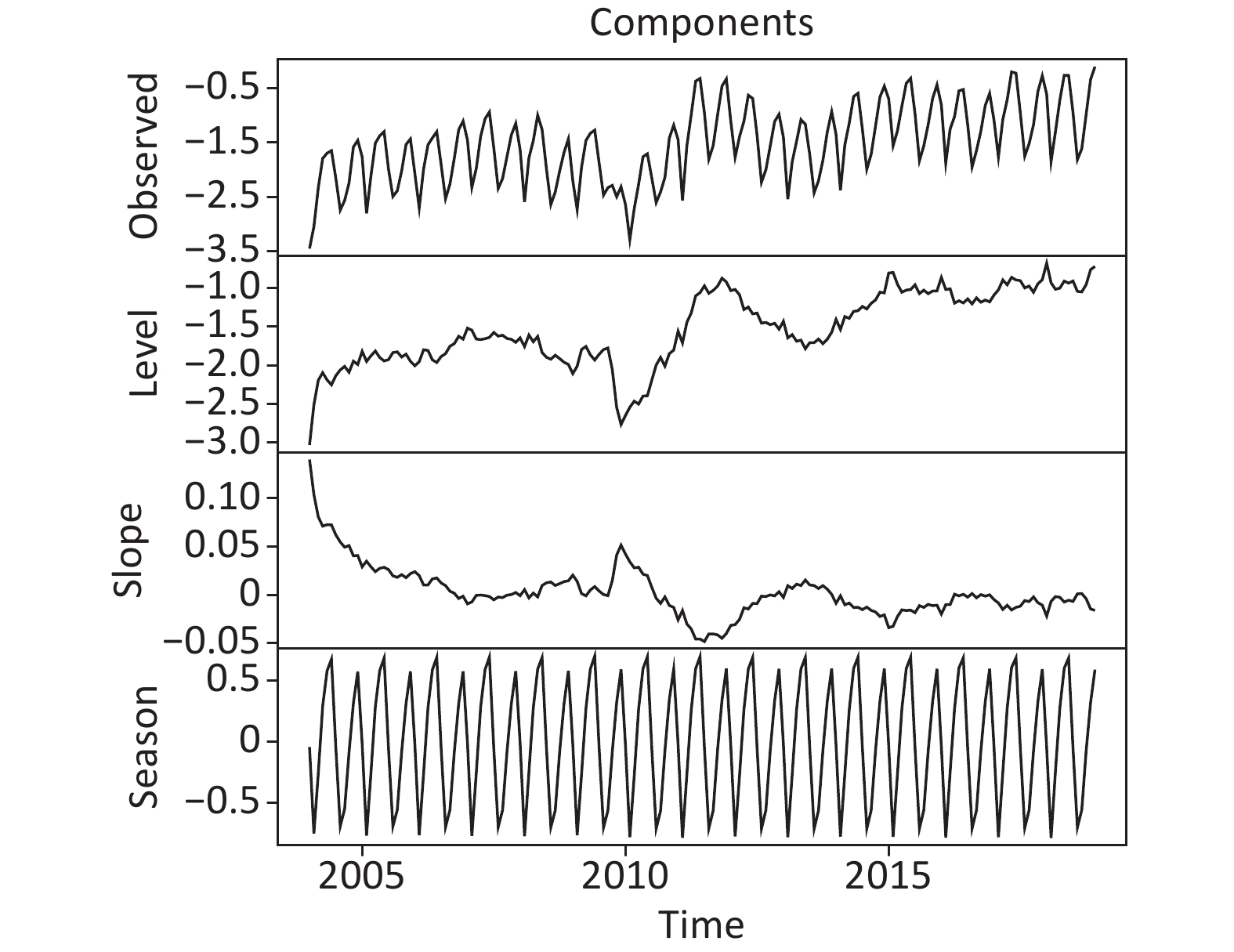
Figure S6. The extracted level, slope, and seasonal components of the best TBATS method developed on the basis of the data from January 2004 to December 2017.
Lags SARIMA (0,1,0)(0,1,1)12 model TBATS(0.01, {0,0}, 0.898, {<12,5>}) model Box-Ljung Q P LM-test P Box-Ljung Q P LM-test P 1 0.024 0.878 0.000 0.993 0.018 0.892 44.923 < 0.001 3 2.353 0.503 2.196 0.533 9.428 0.024 17.323 < 0.001 6 4.529 0.605 4.287 0.638 27.713 < 0.001 18.742 0.005 9 7.720 0.563 6.063 0.734 35.665 < 0.001 22.380 0.008 12 15.292 0.226 9.747 0.638 39.404 < 0.001 22.715 0.030 15 15.349 0.427 13.651 0.552 48.268 < 0.001 22.695 0.091 18 15.980 0.594 21.290 0.265 53.640 < 0.001 25.463 0.113 21 18.952 0.588 21.569 0.425 70.249 < 0.001 24.902 0.251 24 24.734 0.420 30.292 0.175 82.013 < 0.001 24.863 0.413 27 27.525 0.436 26.218 0.507 89.634 < 0.001 26.398 0.497 30 27.536 0.595 27.588 0.592 97.136 < 0.001 27.268 0.609 33 29.788 0.628 31.192 0.557 107.120 < 0.001 29.080 0.663 36 42.128 0.223 37.860 0.384 113.480 < 0.001 29.872 0.754 Note. SARIMA seasonal autoregressive integrated moving average method, TBATS an advanced innovation state-space modelling framework by combining Box-Cox transformations, Fourier series with time-varying coefficients and autoregressive moving average (ARMA) error correction. Table S3. The Box-Ljung Q and LM tests for the best SARIMA (0,1,0)(0,1,1)12 model and TBATS (0.01, {0,0}, 0.898, {<12,5>}) model built based on the date from January 2004 to December 2018
Lags SARIMA (0,1,0)(0,1,1)12 model TBATS (0.048, {0,0}, 0.902, {<12,5>}) model Box-Ljung Q P LM-test P Box-Ljung Q P LM-test P 1 0.055 0.815 0.001 0.975 0.023 0.879 41.160 < 0.001 3 1.921 0.589 2.011 0.570 6.733 0.081 14.042 0.003 6 3.835 0.699 3.951 0.683 22.488 0.001 15.202 0.019 9 6.482 0.691 5.727 0.767 27.233 0.001 18.045 0.035 12 13.434 0.338 8.305 0.761 29.988 0.003 18.208 0.110 15 13.478 0.565 11.083 0.747 35.413 0.002 18.302 0.247 18 14.064 0.725 17.475 0.491 38.712 0.003 21.100 0.274 21 17.679 0.669 17.610 0.674 51.174 0.002 20.863 0.467 24 22.746 0.535 25.236 0.393 60.873 < 0.001 20.972 0.640 27 25.130 0.567 21.988 0.738 65.748 < 0.001 22.446 0.714 30 25.270 0.712 22.799 0.823 70.290 < 0.001 23.178 0.808 33 28.759 0.678 25.691 0.814 78.981 < 0.001 24.382 0.861 36 40.773 0.269 32.064 0.656 83.260 < 0.001 24.538 0.926 Note. SARIMA seasonal autoregressive integrated moving average method, TBATS, an advanced innovation state-space modelling framework by combining Box-Cox transformations, Fourier series with time-varying coefficients and autoregressive moving average (ARMA) error correction. Table S4. The Box-Ljung Q and LM tests for the best SARIMA (0,1,0)(0,1,1)12 model and TBATS (0.048, {0,0}, 0.902, {<12,5>}) model built based on the date from January 2004 to December 2016
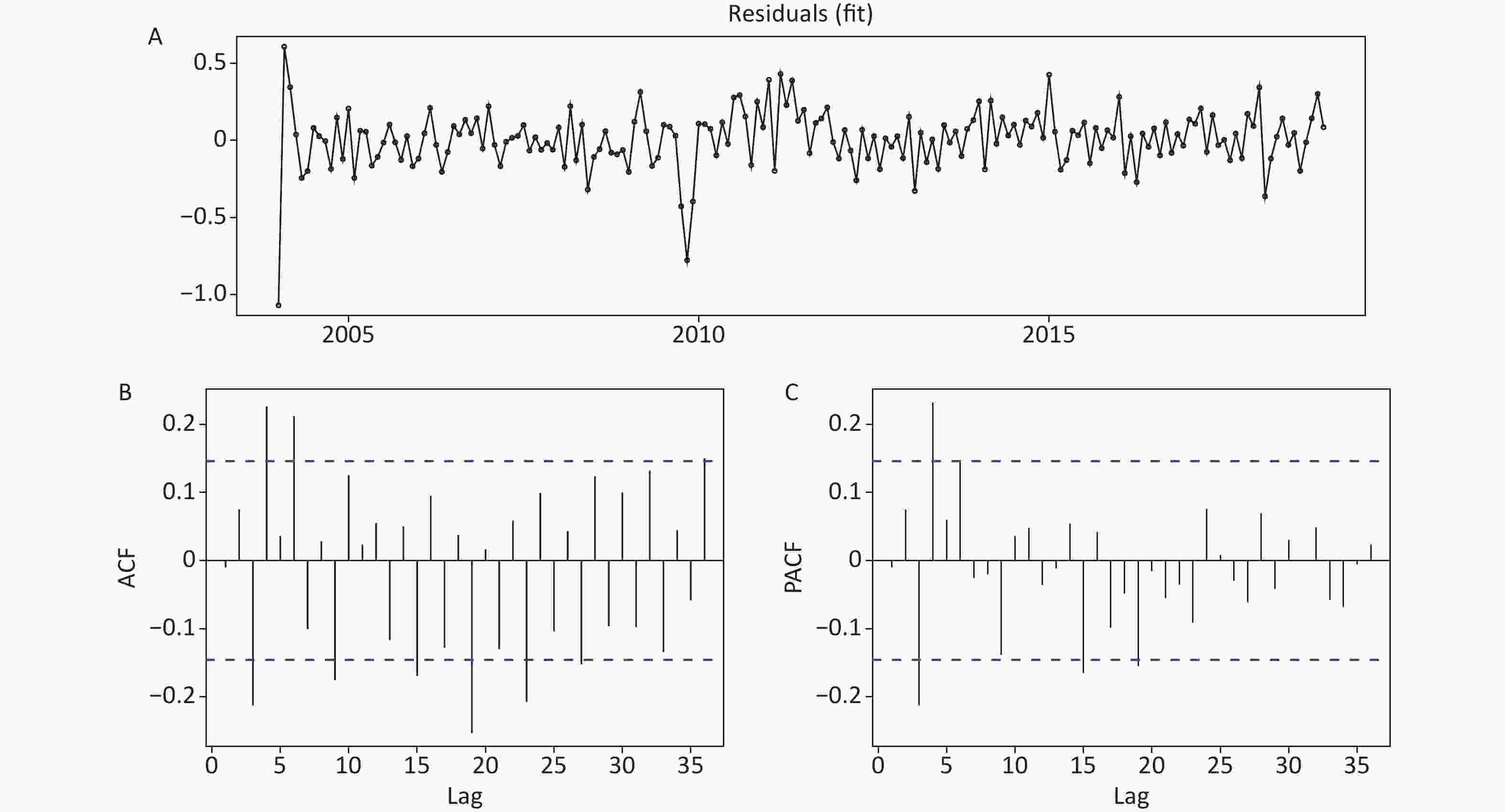
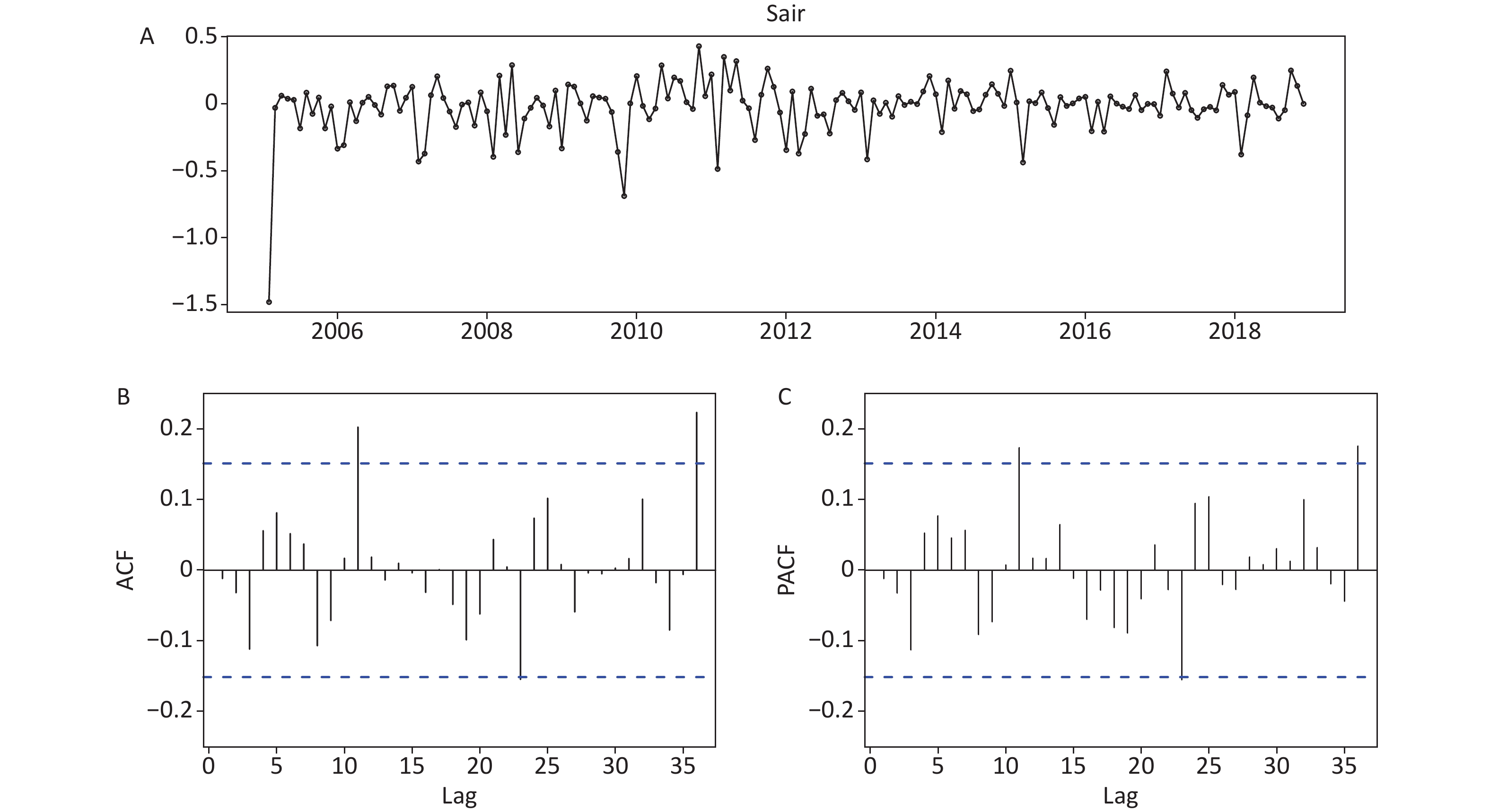
Figure S7. Statistical checking for the residual series of the TBATS model developed on the basis of the data from January 2004 to December 2018. (A) Time series plot showing the residual series. (B) Autocorrelation function (ACF) plot. (C) Partial autocorrelation function (PACF) plot. The correlogram shows that although there are some residual ACF and PACF for the forecast errors that exceed the significance bounds, this is the best model used to estimate the upcoming 12-month epidemics of scarlet fever.

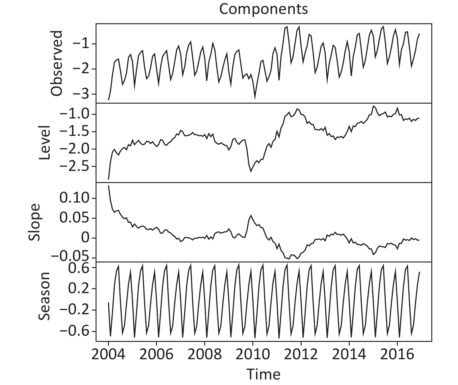
Figure S10. The extracted level, slope, and seasonal components of the best TBATS method developed on the basis of the data from January 2004 to December 2016.
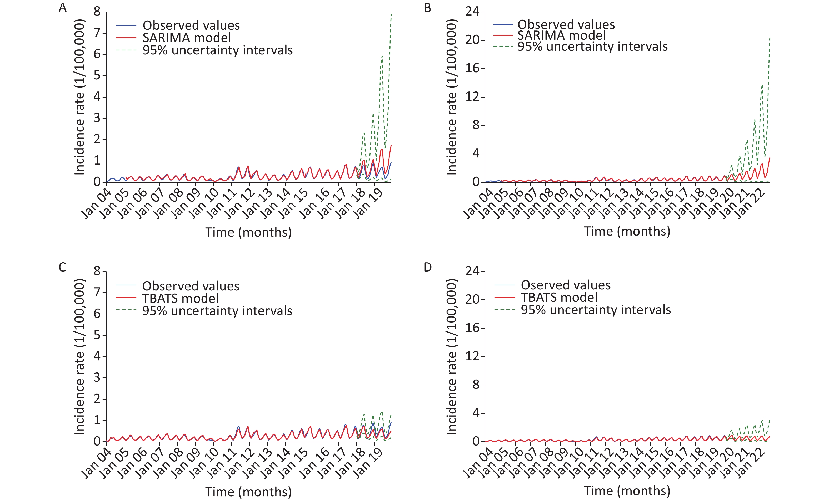
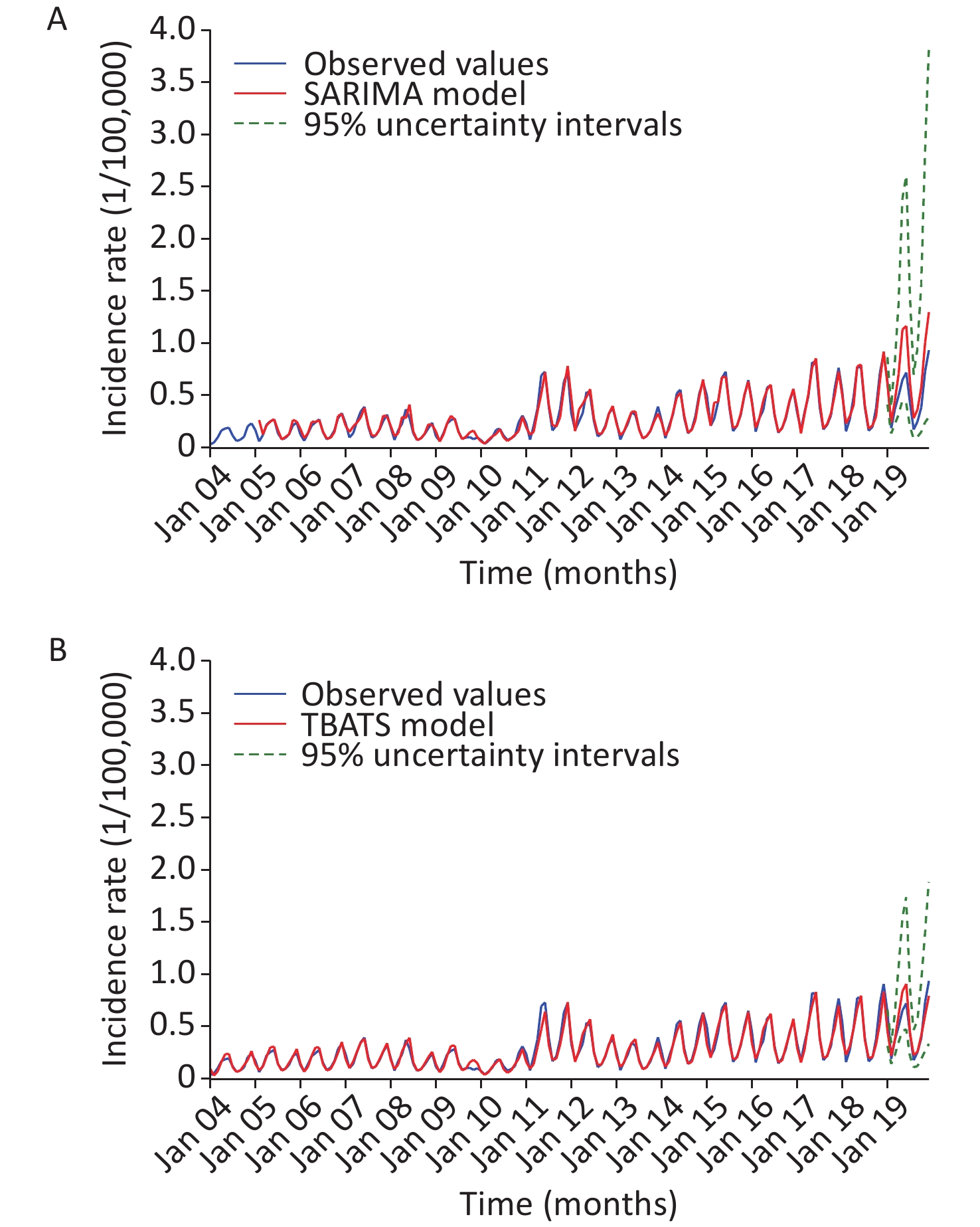
Similarly, following the SARIMA modelling steps, the optimal SARIMA models on different datasets were identified (Supplementary Tables S2–S5, and Supplementary Figures S5, S11–S12, available in www.besjournal.com). Subsequently, the best SARIMA and TBATS models could be used to perform multistep ahead predictions (Figure 1 and Supplementary Figures S13–S14, available in www.besjournal.com). Table 1 lists the measurement metrics, which indicate the forecasting reliability levels on different time windows under the preferred SARIMA and TBATS models. The optimal TBATS models provided a smaller MAD, MAPE, RMSE, RMSPE, and MER compared with the optimal SARIMA models, with a performance improvement of almost 50% in the forecasting abilities for estimating both short- and long-term epidemiological trends, albeit the predictive potential showed a slight reduction with the increase in prediction time windows. We further compared the forecasting abilities of both methods for 48- and 72-step ahead predictions, and the comparative results are listed in Supplementary Tables S1, S6–S7, and Supplementary Figures S15–S16 (available in www.besjournal.com), which show a similar finding, but the predictive results deviated from the epidemic trajectories. In addition, we used the SF incidence data in Liaoning, Heilongjiang, and Shandong provinces, and Inner Mongolia (which are the hardest hit areas by SF in China in the last decade [2, 3]) to assess the predictive quality of these two methods. Likewise, the TBATS method produced lower error rates in all the datasets (Supplementary Table S8, available in www.besjournal.com). Our recent study indicated that the Error-Trend-Seasonal (ETS) model also has a powerful potential in estimating the long-term epidemic behaviors of diseases [4]. As a result, we further developed the ETS model based on the SF morbidity to predict the epidemiological trends, and the results also showed similar findings (the computed MAPE values were 16.101% vs. 38.511%, 21.142% vs. 28.273%, and 23.984% vs. 26.735% in the 12-, 24-, and 36-step ahead forecasts, respectively; Supplementary Table S9, available in www.besjournal.com). These findings further substantiated the utility of the TBATS model. The TBATS model was introduced by adding the trigonometric representation of seasonal components based on the Fourier series into the traditional BATS model, which enabled handling of all complex time series, as well as linear and non-linear information [5], thus indicating the suitability and adequacy of this model. Considering the attractive advantages of the TBATS model, this model can be recommended as a flexible and useful long-term predictive tool in assessing the epidemic patterns of SF in other countries or other contagious diseases; however, further work is required for validation. Moreover, with the rapid advances in the forecasting domain of time series, many hybrid prediction models (e.g., SARIMA-BPNN, SARIMA-GRNN, and SARIMA-LSTM) have also been reported to show an attractive advantage in estimating the long-term epidemic trajectories of diseases. Therefore, what is now needed are studies involving comparisons of the predictive reliable level between the TBATS model and the above-mentioned models.
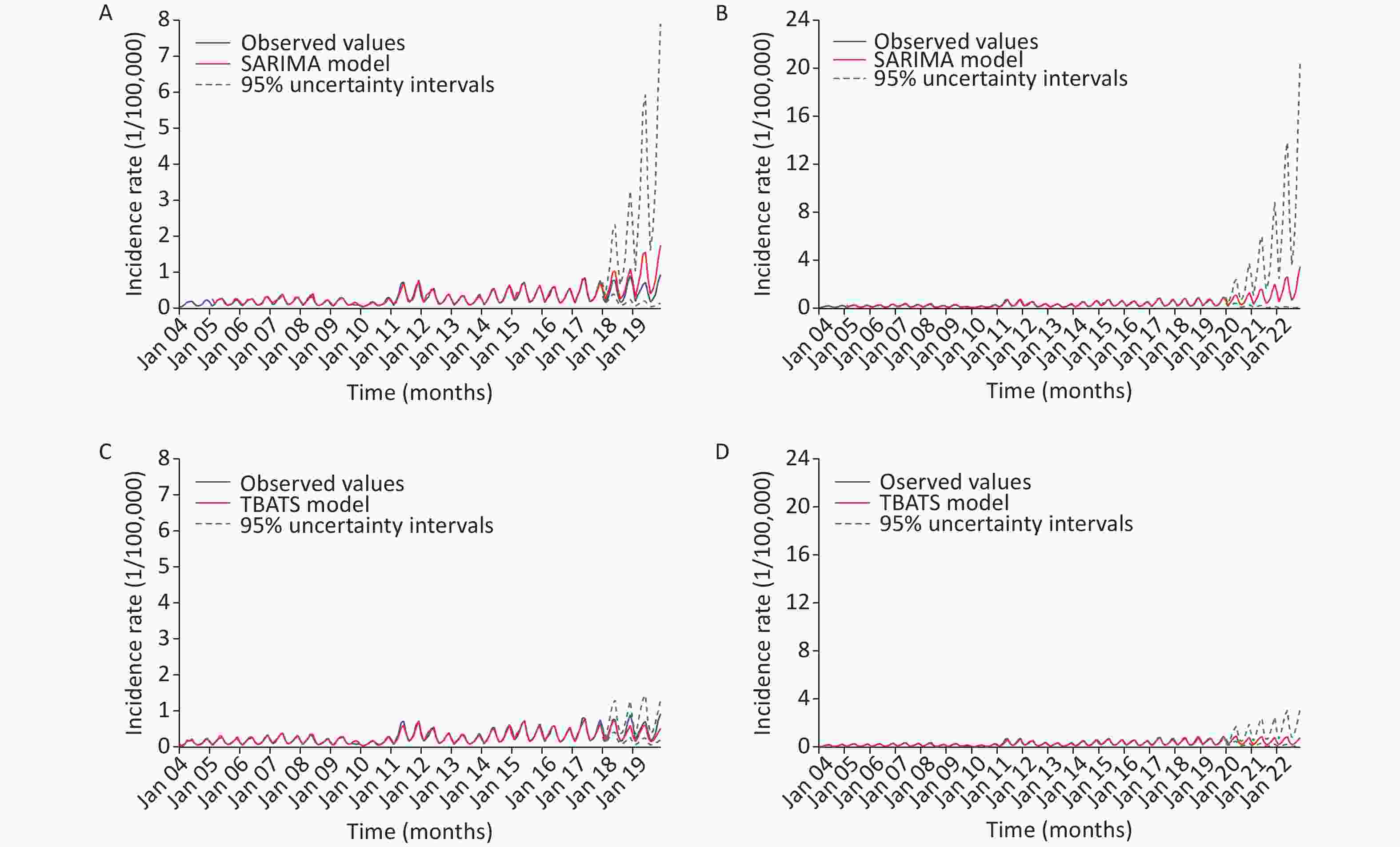
Figure 1. Comparative results of the forecasts based on the SARIMA and TBATS models. (A) The comparison between the 24-step ahead forecasts of the SARIMA model and the observed values. (B) The predicted upcoming 36-month values from January 2020 to December 2022 using the SARIMA model. (C) The comparison between the 24-step ahead forecasts of the TBATS model and the observed values. (D) The predicted upcoming 36-month values from January 2020 to December 2022 using the TBATS model.
Models Testing horizons MAD MAPE RMSE MER RMSPE 24-step ahead predictions SARIMA 0.295 64.346 0.382 0.607 0.551 TBATS 0.114 21.142 0.160 0.235 0.061 Reduced percentage (%) SARIMA vs. TBATS 61.356 67.143 58.115 61.285 88.929 12-step ahead predictions SARIMA 0.212 42.951 0.257 0.429 0.467 TBATS 0.087 16.101 0.113 0.177 0.193 Reduced percentage (%) SARIMA vs. TBATS 58.962 62.513 56.031 58.741 58.672 36-step ahead predictions SARIMA 0.258 55.527 0.396 0.546 0.758 TBATS 0.133 23.984 0.174 0.282 0.271 Reduced percentage (%) SARIMA vs. TBATS 48.450 56.807 56.061 48.352 64.248 Note. SARIMA, seasonal autoregressive integrated moving average method; TBATS, an advanced innovation state-space modelling framework by combining Box-Cox transformations, Fourier series with time-varying coefficients and autoregressive moving average (ARMA) error correction; MAD, mean absolute deviation; MAPE, mean absolute percentage error; RMSE, root mean square error; MER, mean error rate; RMSPE, root mean square percentage error. Table 1. The comparisons of the predicted results between the SARIMA model and the TBATS model on different testing datasets
Variables Estimate S.E. t P Stationary R2 R2 AIC BIC Ljung-Box Q (18) Statistics P SARIMA (0,1,0)(0,1,1)12method developed on the basis of the data from January 2004 to December 2018 SMA1 0.782 0.072 10.873 < 0.001 0.300 0.944 −6.159 −6.146 15.980 0.525 SARIMA (0,1,0)(0,1,1) 12 method developed on the basis of the data from January 2004 to December 2017 SMA1 0.795 0.075 10.600 < 0.001 0.292 0.935 −6.166 −6.152 13.663 0.691 SARIMA (0,1,0)(0,1,1) 12 method developed on the basis of the data from January 2004 to December 2016 SMA1 0.771 0.084 9.230 < 0.001 0.288 0.922 −6.162 −6.127 14.064 0.663 Note. SARIMA seasonal autoregressive integrated moving average method, S.E. standard error, AIC Akaike's Information Criterion, BIC Schwarz's Bayesian Information Criterion, SMA1 seasonal moving average method at lag 1. Table S5. The obtained best SARIMA models with their key parameters on the basis of different datasets
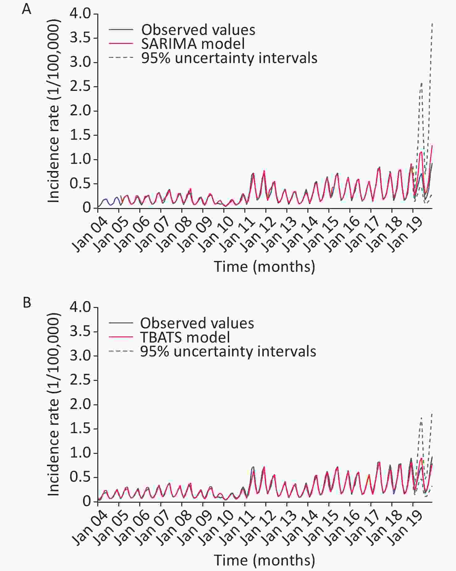
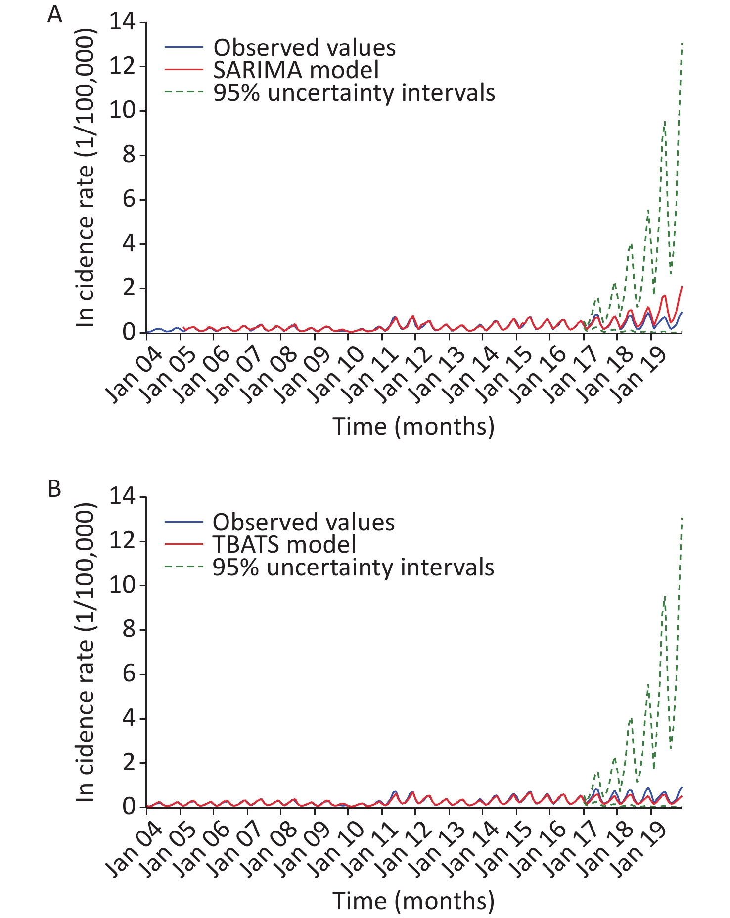
Figure S13. Comparative results of the forecasts based on the SARIMA and TBATS models. (A) The comparison between the 12-step ahead forecasts of the SARIMA model and the observed values. (B) The comparison between the 12-step ahead forecasts of the TBATS model and the observed values.
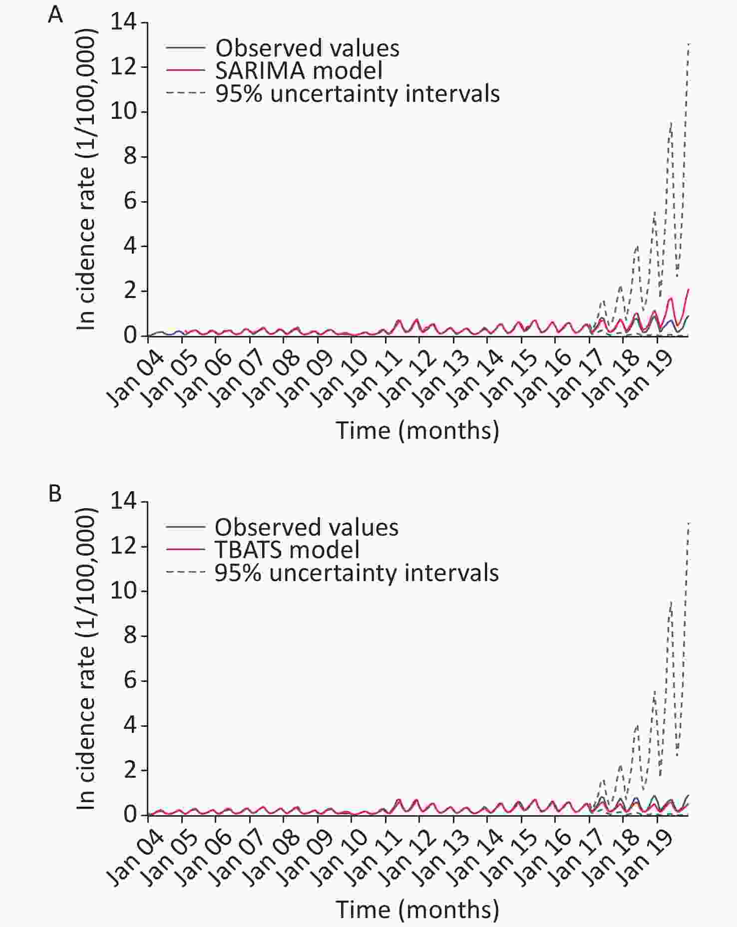
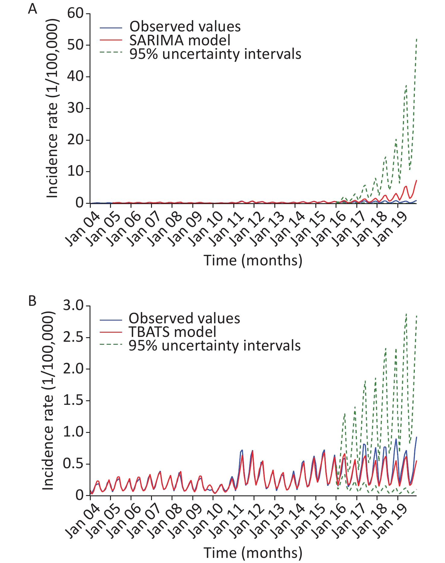
Figure S14. Comparative results of the forecasts based on the SARIMA and TBATS models. (A) The comparison between the 36-step ahead forecasts of the SARIMA model and the observed values. (B) The comparison between the 36-step ahead forecasts of the TBATS model and the observed values.
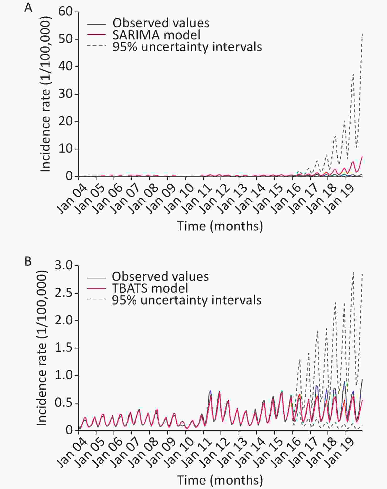
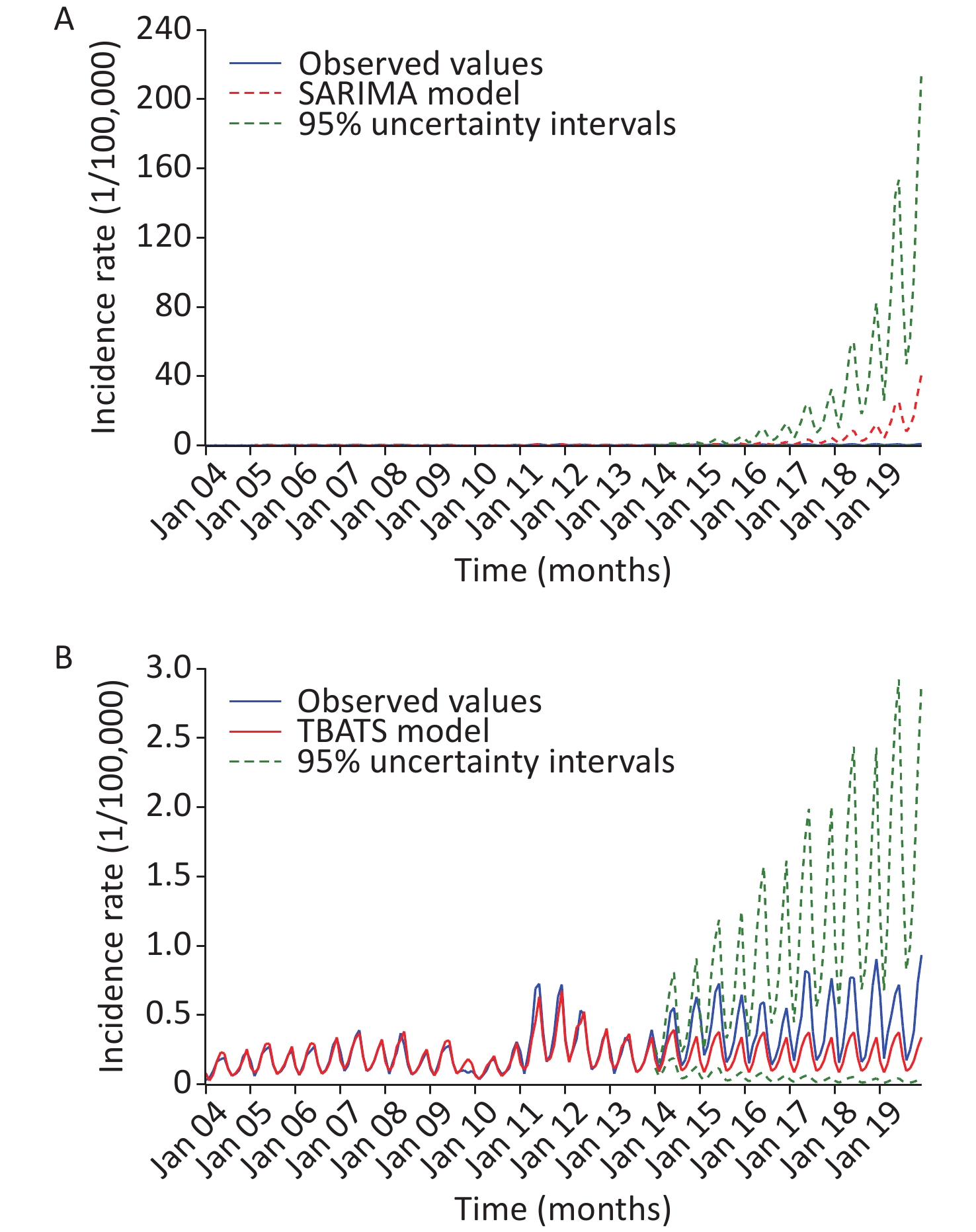
Figure S15. Comparative results of the forecasts based on the SARIMA and TBATS models. (A) The comparison between the 48-step ahead forecasts of the SARIMA model and the observed values. (B) The comparison between the 48-step ahead forecasts of the TBATS model and the observed values.
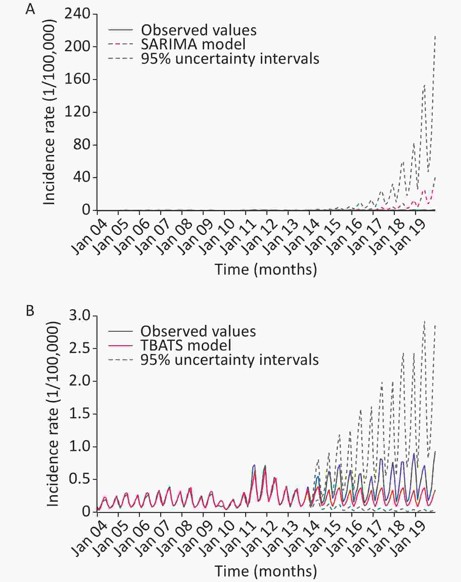
Figure S16. Comparative results of the forecasts based on the SARIMA and TBATS models. (A) The comparison between the 72-step ahead forecasts of the SARIMA model and the observed values. (B) The comparison between the 72-step ahead forecasts of the TBATS model and the observed values.
Sites Models Testing horizons MAD MAPE RMSE MER Liaoning province 12-step-ahead forecast SARIMA (0,1,0)(0,1,1)12 0.681 8.983 0.858 0.697 TBATS (0.073, {4,0}, 0.888, {<12,4>}) 0.358 5.830 0.432 0.367 Percentage reductions (%) TBATS vs. SARIMA 47.430 35.100 49.650 47.346 24-step-ahead forecast SARIMA (0,1,0)(0,1,1)12 0.330 42.453 0.509 0.326 TBATS(0.121, {0,0}, 0.868, {<12,4>}) 0.262 25.144 0.372 0.259 Percentage reductions (%) TBATS vs. SARIMA 20.606 40.772 26.916 20.552 36-step-ahead forecast SARIMA (0,1,0)(0,1,1)12 2.303 275.181 3.207 2.393 TBATS (0.052, {0,0}, 0.875, {<12,5>}) 0.224 26.448 0.305 0.233 Percentage reductions (%) TBATS vs. SARIMA 90.274 90.389 90.490 90.263 Heilongjiang province 12-step-ahead forecast SARIMA (0,1,0)(0,1,1)12 0.227 51.808 0.262 0.383 TBATS (0.151, {0,0}, 0.889, {<12,5>}) 0.130 32.657 0.167 0.219 Percentage reductions (%) TBATS vs. SARIMA 42.731 36.965 36.260 42.820 24-step-ahead forecast SARIMA (0,1,0)(0,1,1)12 0.402 74.176 0.562 0.655 TBATS (0.17, {0,0}, 0.889, {<12,5>}) 0.119 25.819 0.162 0.194 Percentage reductions (%) TBATS vs. SARIMA 70.398 65.192 71.174 70.382 36-step-ahead forecast SARIMA (0,1,0)(0,1,1)12 1.448 253.072 2.114 2.357 TBATS(0.161, {0,0}, 0.894, {<12,4>}) 0.155 20.235 0.252 0.446 Percentage reductions (%) TBATS vs. SARIMA 89.296 92.004 88.079 81.078 Shandong province 12-step-ahead forecast SARIMA (0,1,1)(0,1,1)12 0.236 39.823 0.282 0.319 TBATS(0, {0,0}, 0.932, {<12,5>}) 0.175 19.390 0.280 0.237 Percentage reductions (%) TBATS vs. SARIMA 25.847 51.310 0.709 25.705 24-step-ahead forecast SARIMA (0,1,1)(0,1,1)12 0.509 76.930 0.670 0.717 TBATS (0, {0,0}, 0.932, {<12,5>}) 0.168 19.222 0.268 0.237 Percentage reductions (%) TBATS vs. SARIMA 66.994 75.014 60.000 66.946 36-step-ahead forecast SARIMA (0,1,1)(0,1,1)12 1.683 246.865 2.376 2.491 TBATS (0, {0,0}, 0.926, {<12,5>}) 0.312 43.277 0.401 0.461 Percentage reductions (%) TBATS vs. SARIMA 81.462 82.469 83.123 81.493 Inner Mongolia 12-step-ahead forecast SARIMA (1,0,2)(0,1,1)12 0.401 51.026 0.496 0.397 TBATS (0.232, {0,0}, -, {<12,4>}) 0.130 32.657 0.167 0.219 Percentage reductions (%) TBATS vs. SARIMA 67.581 35.999 66.331 44.836 24-step-ahead forecast SARIMA (1,0,2)(0,1,1)12 0.319 38.984 0.418 0.308 TBATS (0.232, {0,0}, -, {<12,4>}) 0.166 16.508 0.236 0.161 Percentage reductions (%) TBATS vs. SARIMA 47.962 57.654 43.541 47.727 36-step-ahead forecast SARIMA (1,0,2)(0,1,1)12 0.484 56.502 0.573 0.494 TBATS (0.21, {0,0}, -, {<12,4>}) 0.158 17.002 0.224 0.161 Percentage reductions (%) TBATS vs. SARIMA 67.355 69.909 60.908 67.409 Note. SARIMA seasonal autoregressive integrated moving average method, TBATS an advanced innovation state-space modelling framework by combining Box-Cox transformations, Fourier series with time-varying coefficients and autoregressive moving average (ARMA) error correction, MAD mean absolute deviation, MAPE mean absolute percentage error, RMSE root mean square error, MER mean error rate. Table S8. The comparisons of the predicted results between the SARIMA model and the TBATS model on different testing datasets
Models Testing power MAD MAPE RMSE MER RMSPE 12-data ahead forecasting SARIMA 144.734 25.049 161.671 0.203 0.296 TBATS 91.799 14.772 123.653 0.129 0.193 ETS 148.635 25.835 177.092 0.209 0.325 Decreased percentage (%) TBATS vs. SARIMA 36.574 41.028 23.516 36.453 34.797 TBATS vs. ETS 38.239 42.822 30.176 38.278 40.615 24-data ahead forecasting SARIMA 357.734 53.753 406.278 0.460 0.625 TBATS 260.619 38.407 301.441 0.335 0.469 ETS 279.014 44.604 307.731 0.359 0.536 Decreased percentage (%) TBATS vs. SARIMA 27.147 28.549 25.804 27.174 24.960 TBATS vs. ETS 6.593 13.893 2.044 6.685 12.500 36-data ahead forecasting SARIMA 290.782 42.156 365.570 0.334 0.560 TBATS 204.151 28.685 254.418 0.235 0.387 ETS 297.359 44.118 347.689 0.342 0.564 Decreased percentage (%) TBATS vs. SARIMA 29.792 31.955 30.405 29.641 30.893 TBATS vs. ETS 31.345 34.981 26.826 31.287 31.383 60-data ahead forecasting SARIMA 224.931 28.874 310.043 0.258 0.424 TBATS 183.780 21.558 235.665 0.211 0.250 ETS 146.437 16.449 212.028 0.168 0.223 Decreased percentage (%) TBATS vs. SARIMA 18.295 25.338 23.990 18.217 41.038 TBATS vs. ETS -20.319 -23.699 -10.030 -20.379 -10.800 84-data ahead forecasting SARIMA 931.622 134.915 1016.813 1.040 1.679 TBATS 167.432 20.081 204.172 0.187 0.240 ETS 183.777 21.010 227.113 0.205 0.250 Decreased percentage (%) TBATS vs. SARIMA 82.028 85.116 79.920 82.019 85.706 TBATS vs. ETS 8.894 4.422 10.101 8.780 4.000 108-data ahead forecasting SARIMA 1483.868 202.729 1588.876 1.560 2.500 TBATS 208.775 22.849 287.536 0.220 0.310 ETS 268.726 30.177 354.045 0.283 0.386 Decreased percentage (%) TBATS vs. SARIMA 85.930 88.729 81.903 85.897 87.600 TBATS vs. ETS 22.309 24.283 18.785 22.261 19.689 Note. SARIMA seasonal autoregressive integrated moving average method, TBATS an advanced innovation state-space modeling framework by combining Box-Cox transformations, Fourier series with time-varying coefficients and autoregressive moving average error correction, ETS Error-Trend-Seasonal framework, MAD mean absolute deviation, MAPE mean absolute percentage error, RMSE root mean square error, MER mean error rate, RMSPE root mean square percentage error. Table S9. Comparisons of the out-of-sample forecasting powers between TBATS models and SARIMA models, along with ETS models
This study had some limitations. First, SF is a mild illness and has rarely led to death since the 20th century [3]. Therefore, infected individuals with mild clinical manifestations sometimes fail to seek medical aid, resulting in under-reporting and under-diagnosis. Second, to ensure that the model obtained a satisfactory forecasting result, it is important to note that this model should be updated with new incidence data. Third, to investigate whether our TBATS model was adequate for estimating the SF epidemics in other study regions or other infectious diseases, much work is still needed. Finally, integrating the factors influencing the SF epidemics may improve the predictive power. Nevertheless, we are not able to perform such an analysis due to the unavailability of a multivariate TBATS method and SF-related factors.
In summary, SF had dual seasonal behaviors, peaking in May–June and November–December, with a recurrence in 2011 in China; since then it started to be increasing in the SF incidence. The TBATS method was advantageous in analyzing the long-term epidemiological seasonality and trends of SF, which can be considered a useful and flexible alternative to aid stakeholders to develop practical solutions to stop the ongoing spread of SF in China. In addition, we re-established the preferred TBATS (0.023, {0,0}, 0.895, {<12,5>}) specification based on the 16 years of data to predict the SF incidence into 2022, although the SF incidence was predicted to reach a plateau in the next 3 years [Supplementary Tables S1 and S10 (available in www.besjournal.com), and Figure 1], the SF incidence remained at a high level, suggesting that additional or comprehensive interventions must be developed to manage this evolving scenario.
Time Forecasts Lower 95% CI Upper 95% CI Time Forecasts Lower 95% CI Upper 95% CI Jan-20 0.479 0.330 0.695 Jul-21 0.426 0.147 1.204 Feb-20 0.224 0.143 0.349 Aug-21 0.220 0.073 0.647 Mar-20 0.380 0.229 0.627 Sep-21 0.250 0.081 0.751 Apr-20 0.627 0.360 1.085 Oct-21 0.412 0.132 1.249 May-20 0.843 0.463 1.521 Nov-21 0.616 0.195 1.890 Jun-20 0.930 0.489 1.750 Dec-21 0.816 0.254 2.543 Jul-20 0.443 0.221 0.879 Jan-22 0.434 0.130 1.400 Aug-20 0.228 0.108 0.474 Feb-22 0.204 0.059 0.686 Sep-20 0.259 0.119 0.557 Mar-22 0.351 0.100 1.186 Oct-20 0.424 0.190 0.935 Apr-22 0.584 0.166 1.988 Nov-20 0.632 0.275 1.429 May-22 0.791 0.222 2.722 Dec-20 0.835 0.354 1.938 Jun-22 0.878 0.242 3.073 Jan-21 0.443 0.180 1.069 Jul-22 0.421 0.111 1.533 Feb-21 0.208 0.081 0.524 Aug-22 0.218 0.055 0.823 Mar-21 0.357 0.137 0.914 Sep-22 0.248 0.062 0.953 Apr-21 0.593 0.223 1.543 Oct-22 0.409 0.102 1.574 May-21 0.801 0.296 2.126 Nov-22 0.612 0.151 2.369 Jun-21 0.889 0.320 2.412 Dec-22 0.811 0.199 3.172 Note. TBATS an advanced innovation state-space modelling framework by combining Box-Cox transformations, Fourier series with time-varying coefficients and autoregressive moving average (ARMA) error correction, CI, confidence interval. Table S10. Projection into the future 36 months from January 2020 to December 2022 using the best TBATS (0.023, {0,0}, 0.895, {<12,5>}) model
Data Availability All the data supporting the findings of the work are contained within the Supplementary Material (Supplementary Table S11, available in www.besjournal.com).

Figure S8. The extracted level, slope, and seasonal components of the best TBATS method developed on the basis of the data from January 2004 to December 2018.
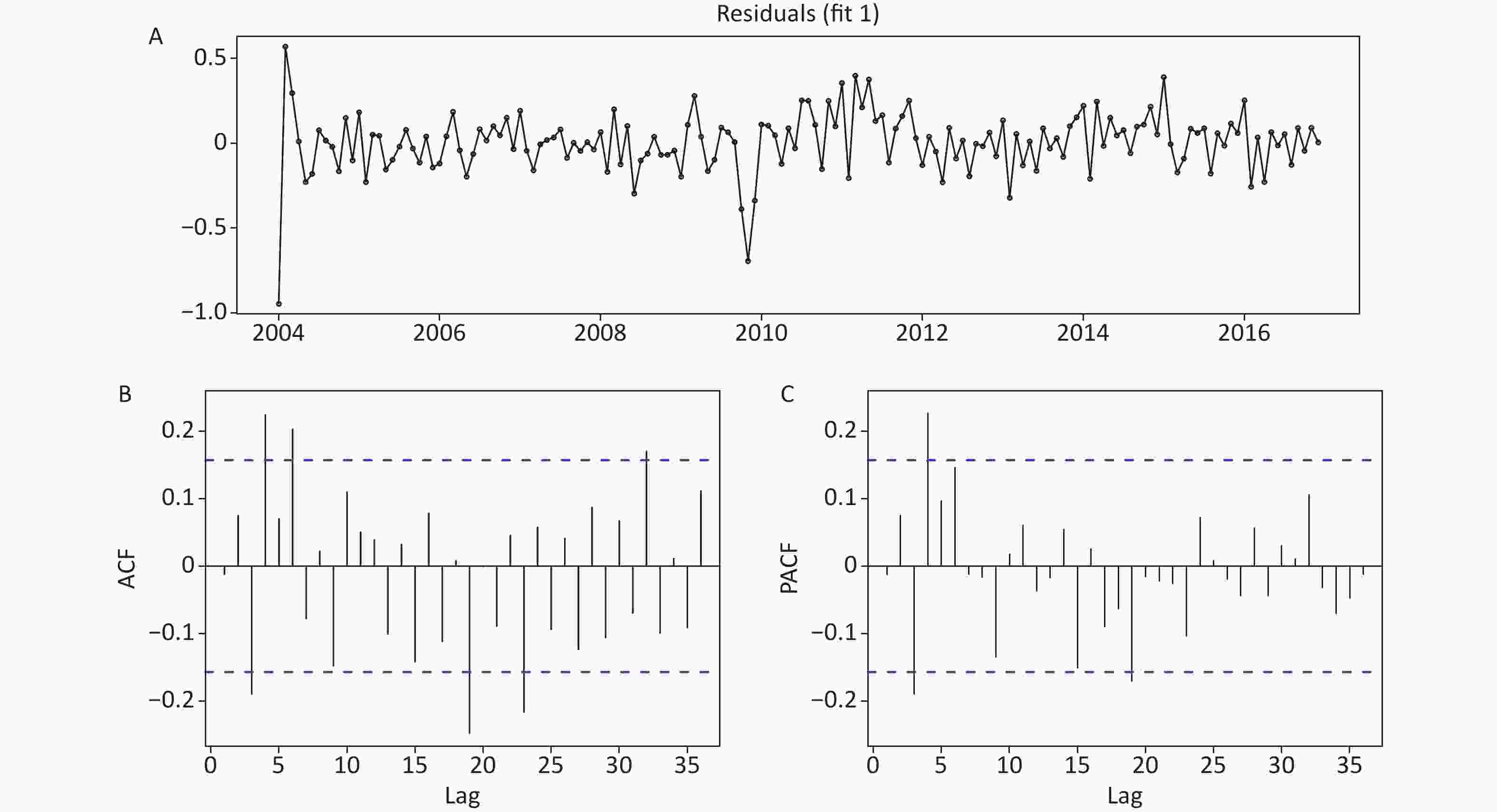
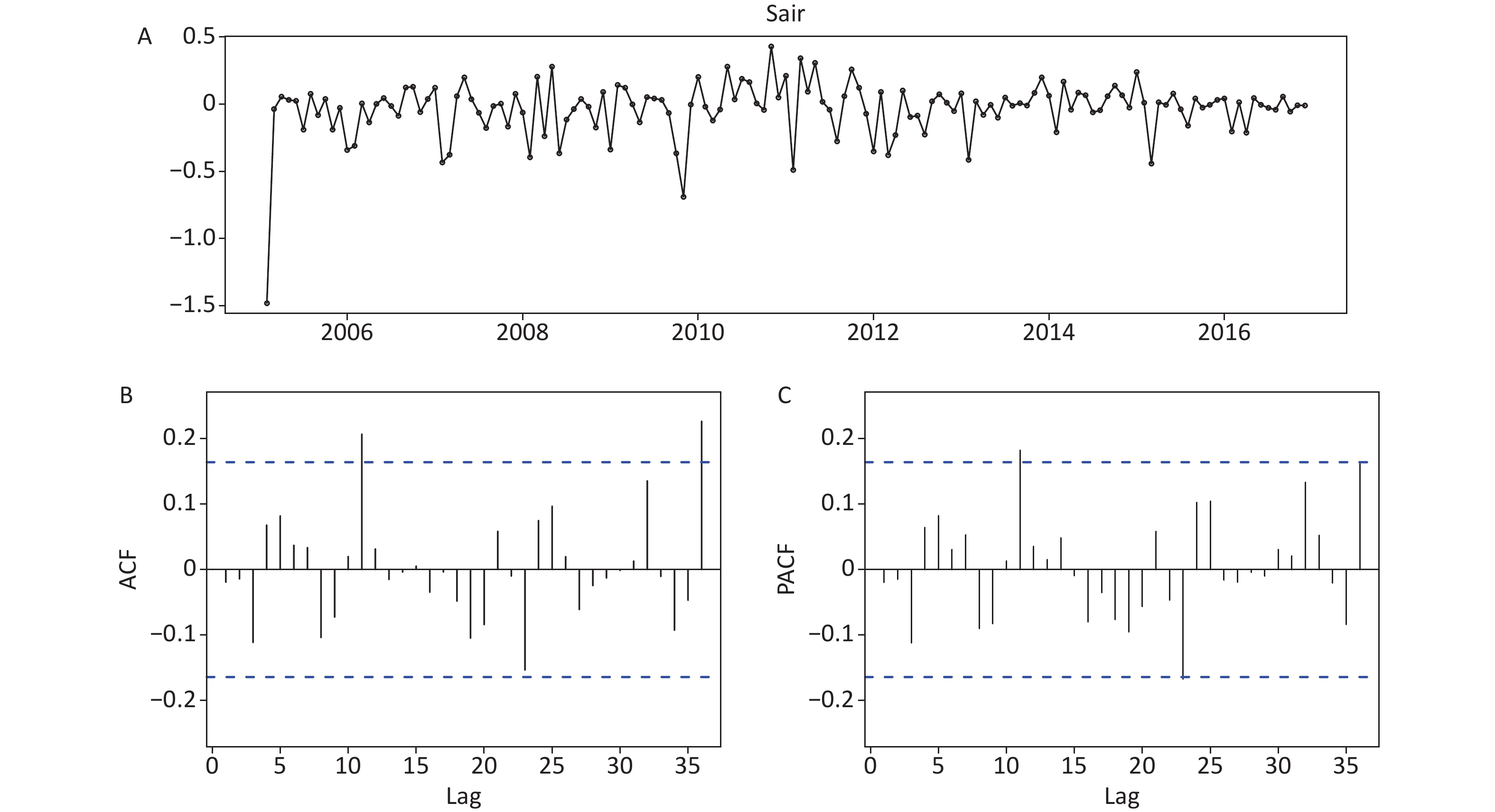
Figure S9. Statistical checking for the residual series of the TBATS model developed on the basis of the data from January 2004 to December 2016. (A) Time series plot showing the residual series. (B) Autocorrelation function (ACF) plot. (C) Partial autocorrelation function (PACF) plot. The correlogram shows that although there are some residual ACF and PACF for the forecast errors that exceed the significance bounds, this is the best model used to estimate the upcoming 36-month epidemics of scarlet fever.
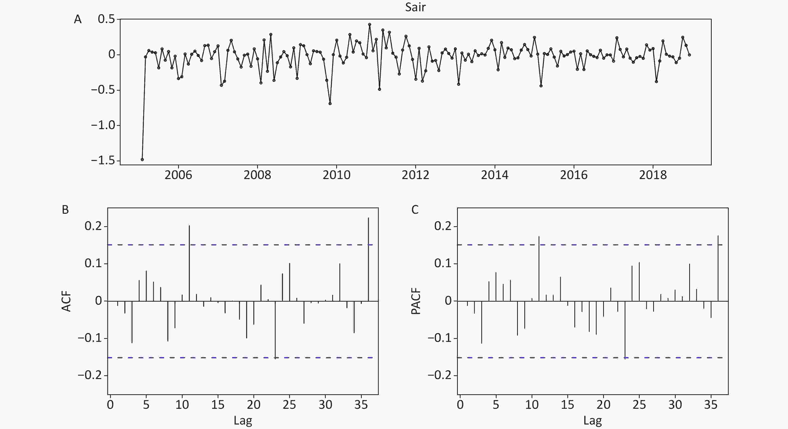
Figure S11. Statistical checking for the residual series of the SSARIMA model developed on the basis of the data from January 2004 to December 2018. (A) Time series plot showing the residual series. (B) Autocorrelation function (ACF) plot. (C) Partial autocorrelation function (PACF) plot. The correlogram shows that the ACF and PACF for the forecast errors do not exceed the significance bounds except for lags 11, 23, and 36, indicating that there is little evidence of non-zero autocorrelations at lags 1–36.
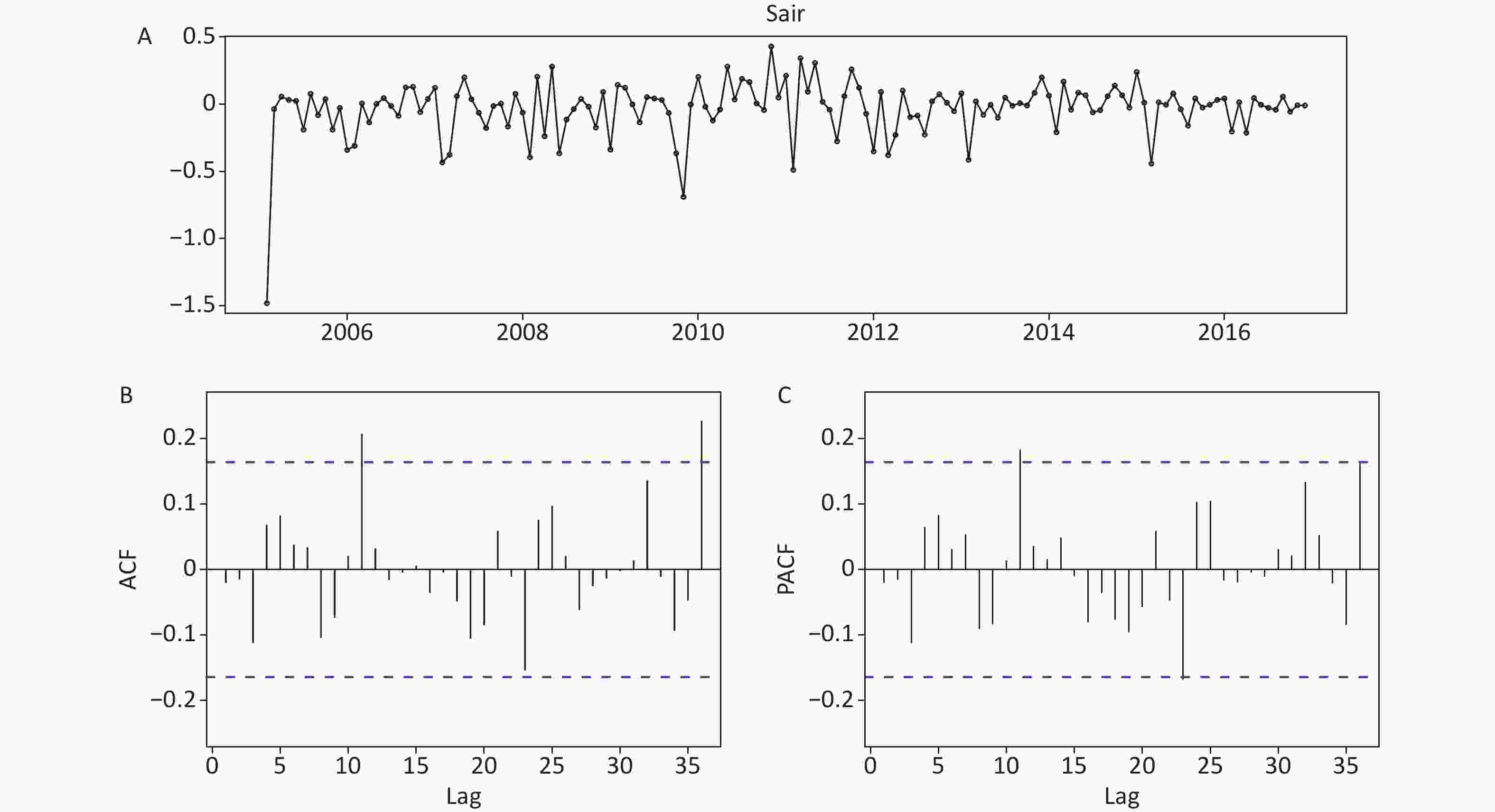
Figure S12. Statistical checking for the residual series of the SARIMA model developed on the basis of the data from January 2004 to December 2016. (A) Time series plot showing the residual series. (B) Autocorrelation function (ACF) plot. (C) Partial autocorrelation function (PACF) plot. The correlogram shows that the ACF and PACF for the forecast errors do not exceed the significance bounds except for lags 11 and 36, indicating that there is little evidence of non-zero autocorrelations at lags 1–36.
Continued Parameters 48-step ahead forecasting 72-step ahead forecasting Future 36-step ahead forecasting TBATS (0.037, {0,0}, 0.901, {<12,5>}) TBATS (0.029, {0,0}, 0.87, {<12,4>}) TBATS (0.023, {0,0}, 0.895, {<12,5>}) Seed states 1 −2.3577 −2.3794 −2.3993 2 0.1062 0.1064 0.1117 3 −0.0314 −0.0546 −0.0067 4 −0.0815 −0.1004 −0.0690 5 −0.0103 −0.0196 −0.0068 6 0.0220 0.0160 0.0300 7 0.0268 0.1411 0.0336 8 0.1425 −0.5940 0.1460 9 −0.5902 −0.0762 −0.6235 10 −0.0647 −0.1476 −0.0634 11 −0.1437 − −0.1522 12 −0.0212 − −0.0232 Sigma 0.1868 0.1947 0.1871 AIC −197.7402 −203.9513 −160.8382 Note. TBATS, an advanced innovation state-space modelling framework by combining Box-Cox transformations, Fourier series with time-varying coefficients and autoregressive moving average (ARMA) error correction, AR autoregressive method, AIC Akaike's Information Criterion. Variables Estimate S.E. t P Stationary R2 R2 AIC BIC Ljung-Box Q (18) Statistics P SARIMA (0,1,0)(0,1,1)12 method developed on the basis of the data from January 2004 to December 2015 SMA1 0.790 0.094 8.394 < 0.001 0.277 0.915 −6.086 −6.072 12.564 0.765 SARIMA (0,1,0)(0,1,1) 12 method developed on the basis of the data from January 2004 to December 2013 SMA1 0.813 0.135 6.025 < 0.001 0.276 0.883 −6.055 −6.032 12.510 0.768 Note. SARIMA seasonal autoregressive integrated moving average method, S.E. standard error, AIC Akaike's Information Criterion, BIC Schwarz's Bayesian Information Criterion, SMA1 seasonal moving average method at lag 1. Table S6. The obtained best SARIMA methods with their key parameters on the basis of different datasets
Models Testing horizons MAD MAPE RMSE MER RMSPE 48-step ahead predictions SARIMA 1.186 252.348 1.850 2.670 3.440 TBATS 0.098 18.307 0.139 0.220 0.222 Reduced percentage (%) SARIMA vs. TBATS 91.737 92.745 92.486 91.760 93.547 72-step ahead predictions SARIMA 0.800 171.381 1.511 1.901 2.810 TBATS 0.207 46.042 0.248 0.491 0.477 Reduced percentage (%) SARIMA vs. TBATS 74.125 73.135 83.587 74.171 83.025 Note. SARIMA seasonal autoregressive integrated moving average method, TBATS an advanced innovation state-space modelling framework by combining Box-Cox transformations, Fourier series with time-varying coefficients and autoregressive moving average (ARMA) error correction, MAD mean absolute deviation, MAPE mean absolute percentage error, RMSE root mean square error, MER mean error rate, RMSPE root mean square percentage error. Table S7. The comparisons of the predicted results between the SARIMA model and the TBATS model on different testing datasets
Date Incidence Date Incidence Date Incidence Date Incidence Date Incidence Date Incidence 01-2004 0.0298 09-2006 0.101 05-2009 0.2623 01-2012 0.3294 09-2014 0.1772 05-2017 0.8192 02-2004 0.0452 10-2006 0.1647 06-2009 0.2782 02-2012 0.1675 10-2014 0.3011 06-2017 0.8006 03-2004 0.0945 11-2006 0.2809 07-2009 0.1508 03-2012 0.2466 11-2014 0.5149 07-2017 0.3811 04-2004 0.1639 12-2006 0.3291 08-2009 0.0821 04-2012 0.3281 12-2014 0.6298 08-2017 0.1711 05-2004 0.1809 01-2007 0.231 09-2009 0.0946 05-2012 0.5325 01-2015 0.499 09-2017 0.2162 06-2004 0.1896 02-2007 0.095 10-2009 0.0988 06-2012 0.5018 02-2015 0.2079 10-2017 0.3078 07-2004 0.113 03-2007 0.1356 11-2009 0.0798 07-2012 0.2523 03-2015 0.2756 11-2017 0.5717 08-2004 0.0619 04-2007 0.2474 12-2009 0.0961 08-2012 0.1047 04-2015 0.4342 12-2017 0.7641 09-2004 0.0742 05-2007 0.3435 01-2010 0.069 09-2012 0.1323 05-2015 0.6642 01-2018 0.5421 10-2004 0.103 06-2007 0.39 02-2010 0.0353 10-2012 0.2071 06-2015 0.7269 02-2018 0.1547 11-2004 0.2033 07-2007 0.1992 03-2010 0.0636 11-2012 0.3264 07-2015 0.3765 03-2018 0.2705 12-2004 0.2299 08-2007 0.0932 04-2010 0.1008 12-2012 0.3741 08-2015 0.1568 04-2018 0.4862 01-2005 0.1686 09-2007 0.1122 05-2010 0.1692 01-2013 0.2437 09-2015 0.2076 05-2018 0.7702 02-2005 0.0582 10-2007 0.1695 06-2010 0.1788 02-2013 0.0762 10-2015 0.3096 06-2018 0.768 03-2005 0.1182 11-2007 0.2543 07-2010 0.1138 03-2013 0.1536 11-2015 0.5007 07-2018 0.3859 04-2005 0.2182 12-2007 0.3153 08-2010 0.0714 04-2013 0.2258 12-2015 0.6459 08-2018 0.1602 05-2005 0.2504 01-2008 0.193 09-2010 0.0872 05-2013 0.3381 01-2016 0.4449 09-2018 0.1967 06-2005 0.2707 02-2008 0.0724 10-2010 0.1149 06-2013 0.3106 02-2016 0.15 10-2018 0.3738 07-2005 0.1344 03-2008 0.1655 11-2010 0.2399 07-2013 0.1756 03-2016 0.2843 11-2018 0.7114 08-2005 0.0801 04-2008 0.2286 12-2010 0.3053 08-2013 0.0858 04-2016 0.3584 12-2018 0.9025 09-2005 0.0891 05-2008 0.367 01-2011 0.2333 09-2013 0.1077 05-2016 0.5771 01-2019 0.6313 10-2005 0.1296 06-2008 0.2816 02-2011 0.0742 10-2013 0.158 06-2016 0.5923 02-2019 0.1851 11-2005 0.2129 07-2008 0.1343 03-2011 0.2074 11-2013 0.2689 07-2016 0.3078 03-2019 0.3657 12-2005 0.2361 08-2008 0.0688 04-2011 0.3728 12-2013 0.3929 08-2016 0.1396 04-2019 0.4974 01-2006 0.1239 09-2008 0.087 05-2011 0.6908 01-2014 0.2568 09-2016 0.1898 05-2019 0.649 02-2006 0.0645 10-2008 0.129 06-2011 0.7253 02-2014 0.0899 10-2016 0.2734 06-2019 0.718 03-2006 0.1345 11-2008 0.1831 07-2011 0.3839 03-2014 0.2113 11-2016 0.4409 07-2019 0.4188 04-2006 0.2117 12-2008 0.2363 08-2011 0.1614 04-2014 0.3171 12-2016 0.5504 08-2019 0.1711 05-2006 0.2406 01-2009 0.1079 09-2011 0.2088 05-2014 0.52 01-2017 0.3333 09-2019 0.2481 06-2006 0.2701 02-2009 0.0625 10-2011 0.369 06-2014 0.5525 02-2017 0.168 10-2019 0.3839 07-2006 0.1454 03-2009 0.1393 11-2011 0.63 07-2014 0.2832 03-2017 0.3394 11-2019 0.7296 08-2006 0.0768 04-2009 0.2292 12-2011 0.7196 08-2014 0.1336 04-2017 0.4895 12-2019 0.9323 Table 11. The SF incidence time series data from January 2004 to December 2019
HTML
Reference
 21432Supplementary Materials.pdf
|

|

 Quick Links
 DownLoad: