Generalized Functional Linear Models: Efficient Modeling for High-dimensional Correlated Mixture Exposures

Humans are exposed to complex mixtures of environmental chemicals and other factors that can affect their health. The importance of studying mixed exposures has been increasingly recognized in recent years^[1,2]. For example, a study on prenatal exposure to multiple endocrine-disrupting chemicals revealed associations with altered cognitive function in children^[3], whereas another investigation revealed that a mixture of air pollutants was linked to increased cardiovascular disease risk⁴. Analyzing the health effects of these multi-pollutant or multi-exposure mixtures presents several key challenges in environmental epidemiology and risk assessment. First, the mixture exposure data are often high-dimensional, with the number of exposures approaching or exceeding the sample size. Second, exposures within a mixture are frequently correlated with each other, leading to issues with multicollinearity in traditional regression models. Third, individual exposures often exert subtle effects that may not be statistically significant on their own. However, when these exposures accumulate in large numbers, they can potentially have a significant effect on health outcomes^[5,6]. The primary goal of mixture exposure studies is to test the overall effect of combined exposure on health outcomes while adjusting for relevant covariates. In many cases, researchers aim to determine the relative contributions of individual exposures within a mixture^[7,8].

Several statistical approaches have been developed to address the challenges in analyzing exposure mixtures. A weighted quantile sum (WQS) regression constructs a weighted index of the mixture components to estimate the overall mixture effect while identifying the relative importance of individual exposures^[9]. WQS is computationally efficient and provides easily interpretable results; however, it assumes that all exposures have effects in the same direction, which may not always be realistic. An extension, known as the two-index WQS, allows for exposures with effects in opposite directions by constructing two separate indices^[10]. This approach provides more flexibility, but may still struggle with highly correlated exposures. Quantile-based g-computation further extends the WQS framework by allowing exposure to effects in opposite directions and providing unbiased estimates of the overall mixture effect^[11]. However, it is based on a generalized linear regression framework and may not fully capture the complex nonlinear exposure-response relationships. Bayesian kernel machine regression (BKMR) can handle high-dimensional data and provides a framework for variable selection. However, its results can be difficult to interpret, and the method is computationally intensive for large datasets^[12].

In this study, we propose a novel statistical approach for analyzing the health effects of exposure mixtures using functional data analysis (FDA) techniques. This method treats the effect of mixture exposure as a smooth function and captures internal correlations to provide meaningful estimation and interpretation. This idea is inspired by approaches used in analyzing single nucleotide polymorphism (SNP) data, which share similarities with mixture exposure data in that individual components may have subtle effects, but their combination can significantly impact outcomes^[13,14]. Our method leverages the strengths of the FDA to handle the high-dimensional and correlation structure inherent in mixture exposure data while allowing for flexible modeling of nonlinear mixture exposure‒response relationships. We developed this approach, conducted extensive simulation studies to evaluate its robustness and efficiency, and applied it to analyze two datasets from the National Health and Nutrition Examination Survey (NHANES). This new framework provides a powerful tool for mixture exposure analysis, offering an improved handling of correlated exposures and interpretable results. It has the potential to advance our understanding of complex environmental exposures and their health impacts, with applications in various fields of environmental epidemiology and toxicology.

Consider $ n $ individuals with measured data for a mixture of $ m $ exposed substances. We assume that the $ m $ exposures are sorted in a random order $ 1 < \cdots < m $ in the collected dataset. For the $ i $ th individual, let $ {y}_{i} $ denote the response of interest, which can be either quantitative or dichotomous, $ {{E}}_{i}={\left({e}_{i1}, \cdots ,{e}_{im}\right)}^{T} $ denote the measured level of $ m $ exposures, and $ {{Z}}_{i}={\left({z}_{i1}, \cdots ,{z}_{ic}\right)}^{T} $ denote the covariates. To relate the exposure mixtures to the response, while adjusting for covariates, we constructed the following model:

in which $ g\left(\cdot \right) $ is an identical link for the quantitative response and logit link for the dichotomous response, $ {\alpha }_{0} $ is the overall mean, $ {\alpha } $ is an $ c\times 1 $ vector of regression coefficients for covariates, and $ \beta \left({x}_{j}\right)\left(j=1, \cdots ,m\right) $ is the exposure effect function (EEF) of position $ {x}_{j} $. Under the functional regression framework, $ \beta \left(x\right) $ is assumed to be a smooth function to reduce the number of coefficients needed to be estimated, whereas, in practice, it is discrete and assumed to be measurable at position $ x $.

Generally, in research studies, there is no inherent order relationship among exposures. These are typically recorded randomly in a dataset, meaning that any two adjacent exposures may be positively, negatively, or uncorrelated. However, Model (1) assumes that the effect of exposure is a smooth function, implying that the arrangement of exposures cannot be random. Consider the following scenario: Suppose that $ {e}_{{j}_{1}} $ and $ {e}_{{j}_{2}} $ are two adjacent exposures in the dataset, where $ {e}_{{j}_{1}} $ is positively correlated with the outcome, but where $ {e}_{{j}_{2}} $ is negatively correlated. In this case, a true effect function needs to transition from a positive to a negative value within a short interval. This is unrealistic for achieving an estimated smooth function without overfitting. Therefore, exposures should be sorted according to a mechanism $ {\Delta } $ to obtain a well-representative effect function $ \beta \left(\cdot \right) $. To mitigate the impact of varying measurement units on effect size estimation, all exposure measurements were transformed into quartiles or decimals. Let $ {{Q}}_{i}(=0, 1, 2, 3) $ denote the quartile version of the exposure data $ {{E}}_{i} $, where $ \left({{\Delta }}_{1}, \cdots ,{{\Delta }}_{m}\right) $ is the new order of the exposure; then, we can use $ {{Q}}_{i}={\left({q}_{i{{\Delta }}_{1}},\cdots ,{q}_{i{{\Delta }}_{m}}\right)}^{T} $ to substitute E_i as

To estimate the EEF $ \beta \left(x\right) $, we can use an ordinary linear square (OLS) smoother¹⁵. Under the OLS framework, let $ {\psi }_{k}\left(t\right),\left(k=1, \cdots ,K,K < m\right) $ be a series of basis functions. Two types of commonly used basis functions are (1) the B-spline basis $ {B}_{k}\left(t\right),k=1, \cdots ,K $ and (2) the Fourier basis $ {F}_{0}\left(t\right)=1,{F}_{2r-1}\left(t\right)=\mathrm{sin}\left(2\pi rt\right), $ and $ {F}_{2r}\left(t\right)=\mathrm{cos}\left(2\pi rt\right),r=1, \cdots ,\left(K-1\right)/2 $. For the Fourier basis, $ K $ is a positive odd integer^15-19. Then, $ \beta \left(x\right) $ can be expanded as

where $ {\Psi } $ is an $ m\times K $ matrix and where $ \mathbf{{\rm B}}={\left({\beta }_{1},\mathrm{ }\cdots ,{\beta }_{K}\right)}^{T} $ is a vector of coefficients. Thus, Model (1) can be rewritten as

in which $ {\mathrm{W}}_{\mathrm{i}}={{Q}}_{i}^{T}{\Psi } $.

Note that

where $ 1 $ is an $ m\times 1 $ vector of size 1. Note that $ {\Psi }\mathbf{{\rm B}} $ is the $ m\times 1 $ vector, $ {1}^{{T}}{\Psi }\mathbf{{\rm B}} $ is the sum of all the elements of $ {\Psi }\mathbf{{\rm B}} $, or the total effect size of mixture exposure, and is the mean change in the outcome when the levels of all the exposures increase by one quartile simultaneously. A 95% confidence interval (CI) was estimated using the bootstrapping method.

The order of exposure significantly influenced the estimation and extrapolation of $ \beta \left(x\right) $. In this study, we propose three common ordering mechanisms, acknowledging that other sorting approaches may be selected based on specific research contexts.

I. Customized Ordering: This method allows researchers to order exposures based on their understanding of the research background. It leverages domain expertise to create meaningful sequences of exposures.

II. Correlation-based Ordering: This approach orders exposures based on their interrelationships, positioning highly correlated variables close to one another. For example, hierarchical clustering can be employed to arrange variables according to the resulting dendrogram. Ordering results can vary significantly depending on the definition of the distance matrix.

i. Define $ 1-\Sigma $, where $ \Sigma $ is the pairwise correlation matrix of exposures, as the distance matrix; then, exposures with high positive correlations are positioned closer, whereas those with strong negative correlations are positioned farther apart.

ii. Define $ 1-\left|\Sigma \right| $ as the distance matrix; then, exposures with strong correlations (either positive or negative) are placed closer together, whereas those with correlations closer to 0 are positioned farther apart.

III. Association-based Ordering: This method orders exposures based on the strength of their associations with an outcome. Variables with similar levels of association with the outcomes were positioned closer to each other.

Unlike traditional regression methods, where multicollinearity can lead to unstable parameter estimates, the GFLM addresses this challenge through its functional smoothing approach. When highly correlated exposures are ordered adjacently, their effects are smoothed together through a basis function expansion, effectively treating them as functional units rather than competing independent variables. This smoothing naturally regularizes the effect estimates, preventing the instability typically observed in standard regression approaches.

Testing the mixture effect of exposures in Model (2) is equivalent to testing hypothesis $ {H}_{0}:\beta \left(x\right)=0\mathrm{v}\mathrm{e}\mathrm{r}\mathrm{s}\mathrm{u}\mathrm{s}{H}_{1}:\beta \left(x\right)\ne 0 $. If $ \beta \left(x\right)=0 $, the outcome is unrelated to the mixture of exposures; otherwise, an association exists. By expanding $ \beta \left(x\right) $ under OLS into Model (4), the test hypothesis is converted to $ {H}_{0}:{{\rm B}}=0\mathrm{v}\mathrm{e}\mathrm{r}\mathrm{s}\mathrm{u}\mathrm{s}{H}_{1}:{{\rm B}}\ne 0 $. This transformation shifts the hypothesis by determining whether a continuous function equals zero when testing finite-dimensional parameters. Based on the testing principle of nested models, we can construct likelihood ratio statistics (LRTs) as

and $ -2\mathrm{ln}\left(\lambda \left({{Q}}^{\text{'}}\right)\right) $ follows an $ {\chi }^{2} $ distribution with degrees of freedom $ K $.

The sequence kernel score test, also known as the global test (GT), is an alternative test statistic suitable for nested models. Within this framework, $ {\alpha } $ in Model (4) is treated as a fixed effect, whereas $ {{\rm B}}={\left({\beta }_{1},\mathrm{ }\cdots ,{\beta }_{K}\right)}^{T} $ is assumed to be an independent and identically distributed random effect, following a normal distribution with a mean of 0 and variance $ {\tau }^{2} $. The test hypothesis is subsequently transformed into $ {H}_{0}:{\tau }^{2}=0\mathrm{v}\mathrm{e}\mathrm{r}\mathrm{s}\mathrm{u}\mathrm{s}{H}_{1}:{\tau }^{2}\ne 0 $. If $ {\tau }^{2}=0 $, each element in $ {{\rm B}} $ equals 0, indicating no association between the exposures and the outcome. Denote $ W={\left({W}_{1}, \cdots ,{W}_{n}\right)}^{T} $, $ {\mathcal{K}}= WW^{T} $, and the variance-component functional kernel score test statistic is

where $ \widehat{\mu } $ and $ {\widehat{\sigma }}_{e}^{2} $ are the predicted mean and variance under the null hypothesis, respectively. That is, $ \widehat{\mu }={\widehat{\alpha }}_{0}+{{Z}}^{T}\widehat{{\alpha }} $, in which $ Z={\left({Z}_{1}, \cdots ,{Z}_{n}\right)}^{T} $ is the covariate matrix, $ {\widehat{\alpha }}_{0} $ and $ \widehat{{\alpha }} $ are the estimations under the null hypothesis; then, $ S\left(\widehat{\mu },{\widehat{\sigma }}_{e}^{2}\right) $ follows a $ {\chi }^{2} $ distribution, which can be approximated by an $ \delta {\chi }_{v}^{2} $ distribution with a degree of freedom $ \nu $ and scale parameter $ \delta $^20-23. Equation (6) is as follows:

in which $ \mu $ and $ {\sigma }_{e}^{2} $ are substituted by $ \widehat{\mu } $ and $ {\widehat{\sigma }}_{e}^{2} $, respectively. According to Kwee et al.²⁴, $ \text{E}\left(S\left(\mu ,{\sigma }_{e}^{2}\right)\right)=tr\left(\mathcal{K}\right) $ can be estimated by $ \widehat{e}=tr\left({P}_{0}\mathcal{K}\right) $, where $ {P}_{0}={I}_{n}-Z{\left({Z}^{T}Z\right)}^{-1}{Z}^{T} $ and where $ {I}_{n} $ is an $ n\times n $ identity matrix. Furthermore, the variance $ Var\left(S\left(\mu ,{\sigma }_{e}^{2}\right)\right)=2tr\left({\mathcal{K}}^{2}\right) $ can be estimated by $ {\widehat{I}}_{\tau \tau }={I}_{\tau \tau }- {I}_{\tau {\sigma }^{2}}^{2}/{I}_{{\sigma }^{2}{\sigma }^{2}}^{2} $, where $ {I}_{\tau \tau }=2tr\left({\left({P}_{0}\mathcal{K}\right)}^{2}\right) $, $ {I}_{\tau {\sigma }^{2}}^{2}=2tr\left({P}_{0}\mathcal{K}{P}_{0}\right) $, and $ {I}_{{\sigma }^{2}{\sigma }^{2}}^{2}=2tr\left({P}_{0}^{2}\right) $. Solving equations $ \delta \nu =\widehat{e} $ and $ 2{\delta }^{2}\nu ={\widehat{I}}_{\tau \tau } $ yields approximations of the scale parameter and the degree of freedom as follows:

An R package implementing GFLM is available at https://github.com/Peng247/Research and can be installed using the R command devtools::install_github ("Peng247/Research").

To evaluate the performance of the GFLM in mixture exposure studies, an extensive simulation study was conducted using the NHANES dataset as the data pool. This approach allows the maintenance of realistic correlation structures and distributions of exposure, thereby providing a more practical assessment of the capabilities of the method. To evaluate GFLM's performance of the GFLM relative to the existing methods, we included WQS regression in the unidirectional simulation scenarios for comparison, as both methods can be directly compared in terms of Type I error control, statistical power, and effect estimation accuracy.

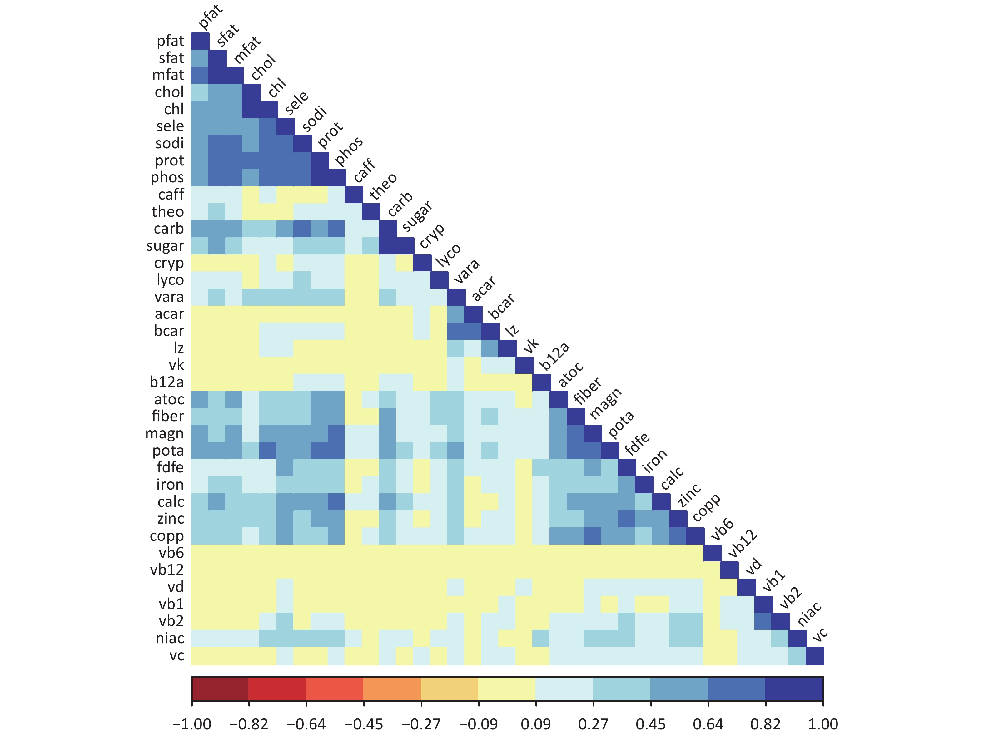
The dataset comprises the 2011–2012, 2013–2014, and 2015–2016 dataset^[10]. The dataset comprised 5,960 adult participants aged 20–60 years, for whom reliable dietary data and complete information on relevant covariates were available. Individuals who had experienced weight loss or other health-related diets at the time of the survey were excluded. The exposure mixture in the data pool consisted of 37 nutrients estimated from dietary intake data collected through two 24-hour dietary recall interviews. These nutrients include a wide range of dietary components such as macronutrients (e.g., carbohydrates, proteins, and various types of fats), vitamins (e.g., vitamins A, complex vitamins, vitamins C, D, E, and K), minerals (e.g., calcium, iron, magnesium, and sodium), and other dietary factors (e.g., fiber and caffeine). The outcome of interest in the original study was obesity, defined as a body mass index (BMI) greater than or equal to 30 kg/m². Approximately 36.2% of individuals in the dataset were classified as obese. The pairwise Spearman correlation coefficients of nutrients are shown in Figure 1, with correlation coefficients ranging from −0.08 to 0.883.

Figure 1.  Spearman correlation matrix among nutrients.

To evaluate the robustness of GFLM, we estimated the empirical type I error rate using a simulation approach. Random samples of 1000, 1500, and 2000 participants were drawn from the original dataset. Within each sample, the order of the outcome variable BMI (both continuous and dichotomous) was randomly permuted to disrupt potential associations with exposures. GFLM were constructed using age and sex as covariates and 37 nutrients as mixture exposures. The significance of the mixture exposure effect was tested using both the LRT and GT.

Given the random permutation of BMI, no significant association between mixture exposure and outcomes was expected. Therefore, the proportion of significant results across simulations provided an estimate of the type-I error rate. Denote $ {P}_{k} $ as the $ p $ value of the $ i $th run of simulation and $ \alpha \text{'} $ as the predetermined significance level; then, the empirical type I error rate after 10⁴ runs is

Under the alternative hypothesis, mixed exposure is associated with the outcome. The continuous outcome is generated by

in which $ {Z}_{1i}~N\left(0, 1\right) $ and $ {Z}_{2i}~Bernoulli\left(0.5\right) $ are continuous and binary covariates, respectively; $ {m}_{+} $ and $ {m}_{-} $ are the numbers of two sets of causal exposures $ {p}_{i} $ and $ {q}_{j} $ with weights $ {v}_{i} $ and $ {u}_{j} $ restricted to $ \sum _{i=1}^{{m}_{+}}{v}_{i}=\sum _{j=1}^{{m}_{-}}{u}_{j}=1 $; $ {w}_{k}\in \left[0, 1\right) $ with $ \sum _{k=1}^{4}{w}_{k}=1 $ are the effect sizes of the corresponding terms; and $ {ϵ}_{i}~N(0, 1) $ are random errors. In Model (7), the negative sign of $ {w}_{4} $ indicates that $ {q}_{j} $ represents exposure with negative effects on the outcome. Given the mutual exclusivity of $ {p}_{i} $ and $ {q}_{j} $, this model assumes a unidirectional association between any single exposure and outcome. The proportion of null-effect exposures can be controlled by adjusting the magnitudes of $ {m}_{+} $ and $ {m}_{-} $. Therefore, $ {w}_{3} $ and $ {w}_{4} $ represent the cumulative positive and negative exposure effects, respectively, and their difference $ {w}_{3}-{w}_{4} $ denoting the overall mixture exposure effect. By setting $ {\alpha }_{0}=\mathrm{log}\left(0.25\right) $, corresponding to a 20% incidence rate, the continuous outcome is generated by $ {y}_{i}~N\left(E\left({y}_{i}\right), 1\right) $, and the binary outcome is generated by $ {y}_{i}~Bernoulli\left(\mathrm{exp}\left\{E\left({y}_{i}\right)\right\}/\left(\mathrm{exp}\left\{E\left({y}_{i}\right)\right\}+1\right)\right) $.

In the empirical power simulation, we focused on two scenarios of interest: unidirectional ($ {w}_{4}=0 $) and bidirectional ($ {w}_{4}\ne 0 $) exposure effects. The effect size was defined as the proportion of the total outcome variance attributable to the mixture exposure effect; 1/3, 1/4, and 1/6 were selected for the simulation. The causal proportion, which represents the ratio of causally active exposures to the total number of exposures in the mixture, was used to model the different patterns of exposure effects. This proportion ranges from 1 (indicating that all exposures are associated with the outcome) to 1/16 (intermediate values of 1/2, 1/4, and 1/8). Sample sizes of 1000, 1500, and 2000 were selected, with 10³ simulation runs for each empirical power calculation. Following the same notation as the empirical type-I error rate, the empirical power is

To demonstrate the practicability of the GFLM, we applied two datasets from the NHANES, each representing a different type of mixture exposure scenario.

The first was the dataset mentioned in the numerical simulation section. The primary objective was to investigate the impact of 37 nutrients on obesity, while controlling for age, sex, race, exercise intensity, and smoking status. Using the GFLM, we tested the significance of the nutrient mixture effect, estimated the magnitude of the overall mixture effect, and quantified the individual contributions of each nutrient.

The second dataset was derived from six NHANES cycles spanning 2007-2018 whose objective was to investigate the association between per- and polyfluoroalkyl substance (PFAS) exposure and gout risk. The initial sample comprised 59,842 participants, which were refined to 7,101 participants through a series of exclusion criteria. The primary outcome (gout status) was determined on the basis of self-reported data collected using a structured questionnaire. The exposure assessment focused on the serum concentrations of four PFAS: perfluorooctanoic acid (PFOA), perfluorooctane sulfonic acid (PFOS), perfluorohexane sulfonic acid (PFHxS), and perfluoronanoic acid (PFNA). These compounds were quantified using online solid-phase extraction coupled with high-performance liquid chromatography-turbo ion spray tandem mass spectrometry. A comprehensive set of covariates was included to adjust for the potential confounding effects. These included demographic variables (age, sex, and ethnicity), socioeconomic factors (educational attainment and family poverty-income ratio), lifestyle factors (smoking status, alcohol consumption, and physical activity level), and health-related variables (BMI). We aimed to test the individual and mixed effects of PFAS on the risk of gout while controlling for various covariates. The detailed sample selection process, definition of outcomes, exposures, covariates, and statistical description of covariates by gout status are presented in Supplementary Information.

The results of the type-I error simulations are listed in Table 1. The dimension reduction rate indicates the intensity of the dimensionality reduction, with 1/2 indicating a reduction of half the original dimensions. In Model (3), the EEF $ \beta \left(x\right) $ is expanded by finite-dimensional basis functions and coefficients $ {\Psi }\mathbf{{\rm B}} $, with the approximation controlled by the number of basis functions $ K $. The dimension reduction rate was calculated as $ K/m $. Smaller $ K $ values represent greater dimensionality reduction, resulting in poorer fitting compared to larger $ K $ values. Table 1 illustrates the robustness of the GFLM in analyzing continuous and binary outcomes under various sample sizes, significance levels, dimensionality reduction intensities, and ordering mechanisms.

Both LRT and GT generally maintain type I error rates close to the nominal significance level $ \alpha $, with GT exhibiting a more conservative tendency. Under association-based ordering, both tests maintain stable control with rates ranging from 0.049-0.059 at $ \alpha =0.05 $. Correlation-based ordering showed slightly more variability in the control group, particularly for the GT with a smaller sample size. The GT was insensitive to the degree of dimensionality reduction, whereas the LRT tended toward an inflated type-I error as the number of mixture exposures increased. For LRT, the robustness of testing continuous outcomes appeared slightly superior to that of binary outcomes, whereas GT demonstrated comparable control across both outcome types. In summary, these findings suggest that the GT provides a more robust testing method for GFLM, maintaining better type-I error control across various scenarios of dimensionality outcome types and ordering mechanisms.

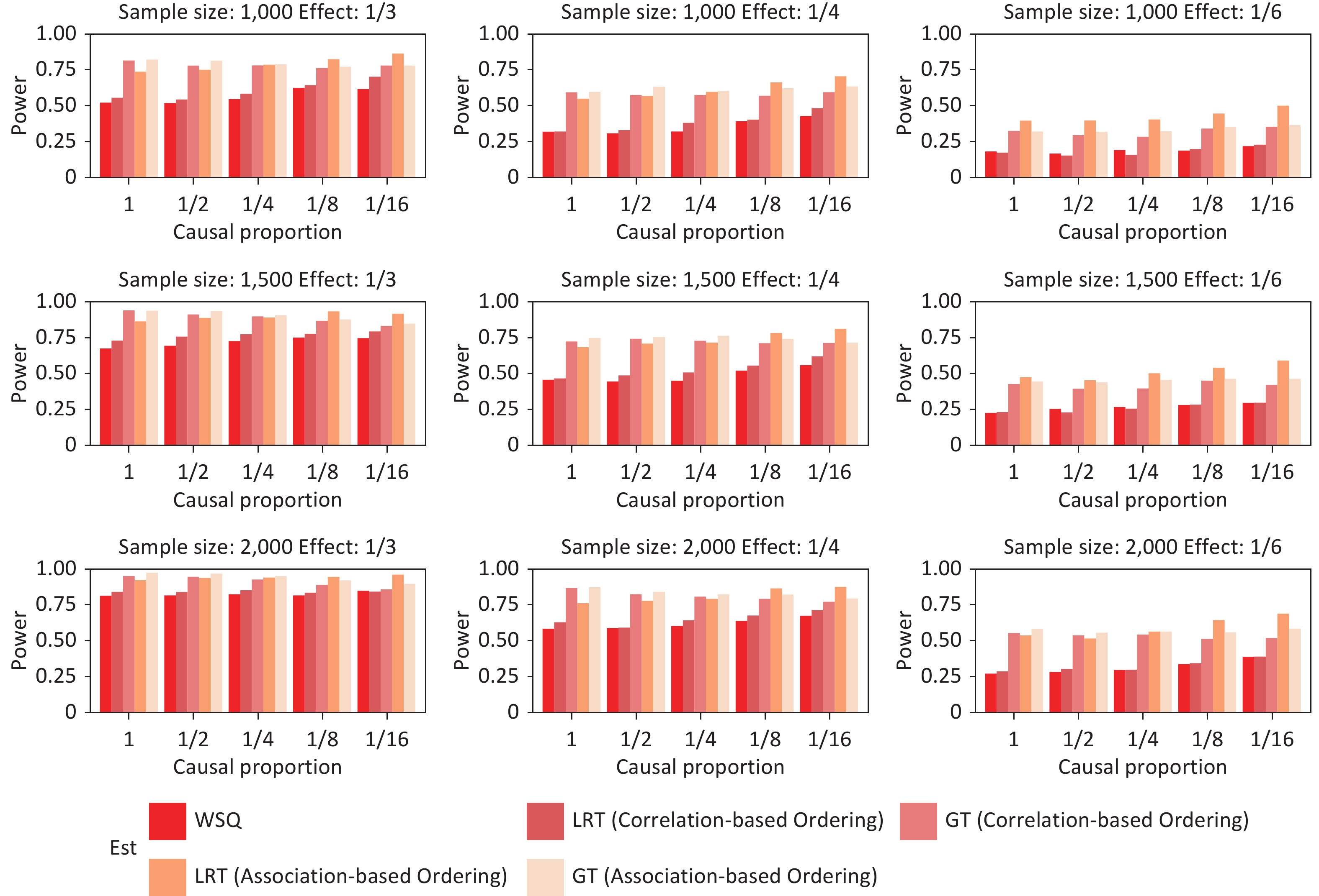
The empirical power of the GFLM was evaluated through extensive simulations, and the results are shown in Figures 2–5. These simulations compared the performances of the LRT and GT under various scenarios, including unidirectional and bidirectional exposure effects for both continuous and binary outcomes.

Figure 2.  Simulation of the unidirectional exposure effect for continuous outcomes under various sample sizes, total effect sizes, causal exposure proportions, and testing method combinations. WQS, weighted quantile sum regression; LRT, likelihood ratio test; GT, global test.

Figure 3.  Power simulation of the unidirectional exposure effect for binary outcomes under various sample sizes, total effect size magnitudes, causal exposure proportions, and testing method combinations. WQS, weighted quantile sum regression; LRT, likelihood ratio test; GT, global test.

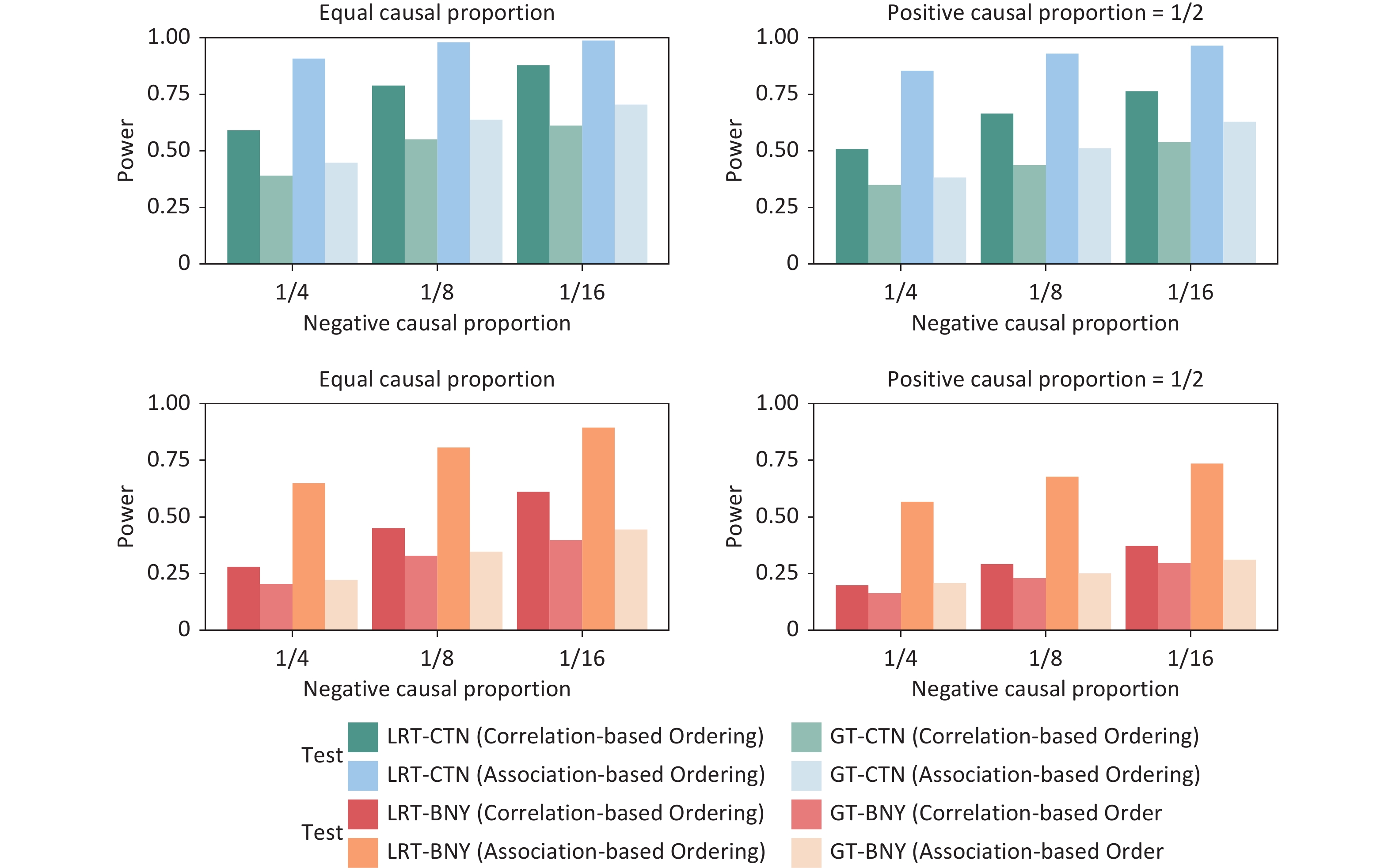
Figure 4.  Power simulation of the bidirectional exposure effect for continuous (first row) and binary (second row) outcomes under various causal proportion combinations when the sample size is fixed to 1500 and when the positive effect size is assumed to be equal to the negative effect size. WQS, weighted quantile sum regression; LRT, likelihood ratio test; GT, global test.

In the unidirectional exposure scenarios (Figure 2–Figure 3), the GFLM demonstrated greater power for continuous outcomes than for binary outcomes. The GT exhibited superior overall performance relative to the LRT, particularly in terms of robustness to effect-size variations. This suggests that the GT may be preferable in situations where the magnitude of the exposure effects is uncertain under the unidirectional assumption of mixture exposure. A comparison with WQS regression reveals that the GFLM provides comparable or superior power across different scenarios, particularly for binary outcomes and smaller effect sizes. While both methods maintain good power for continuous outcomes, the GFLM demonstrates a more stable performance across varying causal proportions. Bidirectional exposure simulations (Figure 4–Figure 5) revealed that the LRT outperformed the GT. This performance difference was particularly pronounced for binary outcomes, particularly when the association-based ordering of exposures was employed. These findings highlight the importance of selecting an appropriate test statistic based on the anticipated direction of the exposure effects and the nature of the outcome variable.

Figure 5.  Power simulation of the bidirectional exposure effect for continuous (the first row) and binary (the second row) outcomes under various causal proportion combinations when the sample size is fixed to 1500 and assuming that the positive effect size is twice the negative effect size. WQS, weighted quantile sum regression; LRT, likelihood ratio test; GT, global test.

In contrast to the intuitive expectation that opposing effects in a mixture would lead to reduced detectability, the simulations demonstrated that the absolute sum of the effect sizes is a key determinant of statistical power. Figure 5 illustrates that regardless of the proportion of positive to negative effects, larger absolute effect sizes consistently yielded greater power. This result underscores the ability of the GFLM to detect significant mixture effects, even in the presence of opposing individual exposure effects.

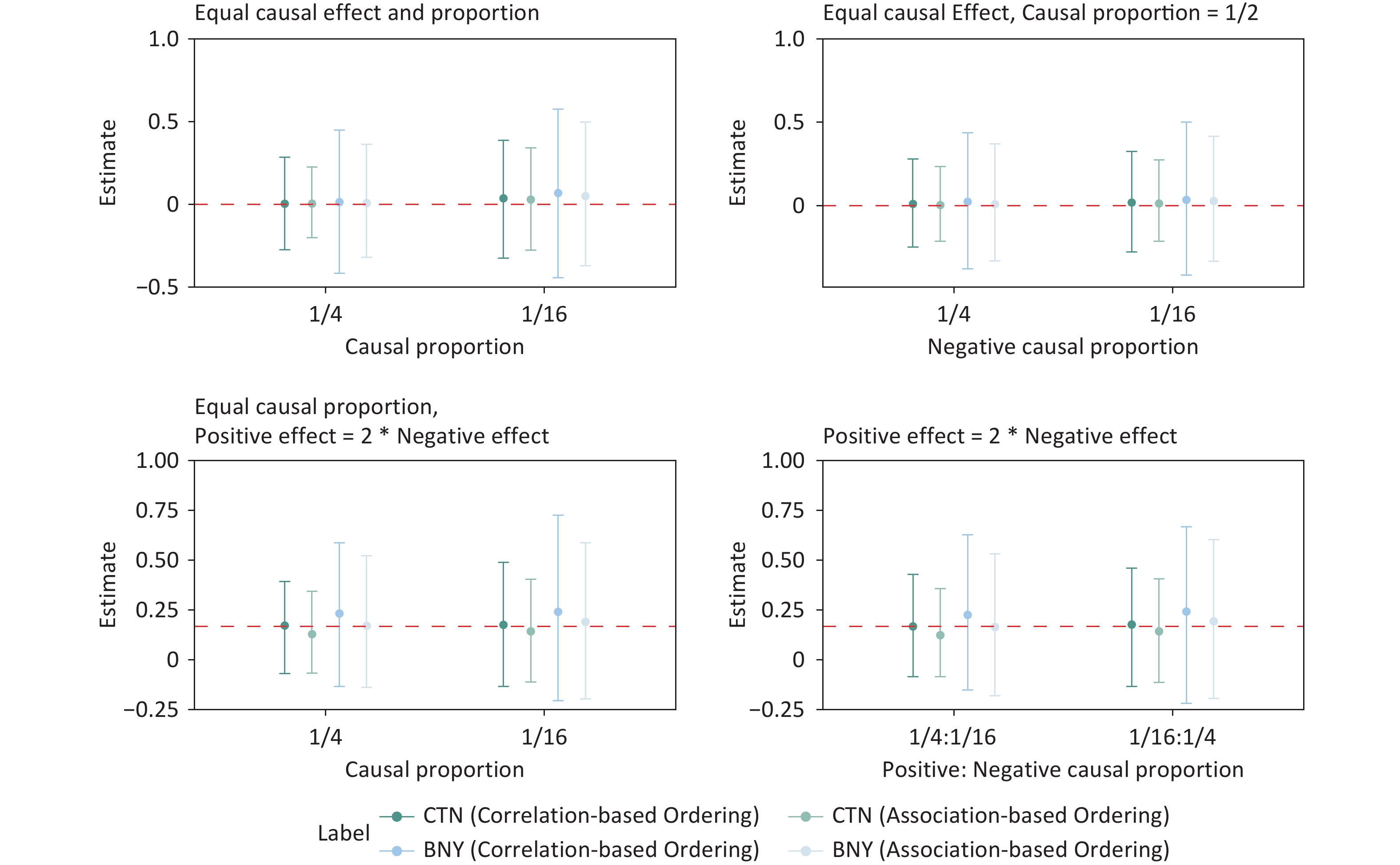
Figure 6 and 7 present the results of effect size estimation for various simulation scenarios. The red dashed line represents the true effect size, and the solid lines represent the 95% confidence intervals for each simulation setting. Across all the simulated scenarios, the 95% CIs consistently encompassed the true effect size, with point estimates generally clustered around the true value. As expected, increasing the sample size reduced the width of the CIs. Figure 6 shows that the GFLM provides more reliable estimates than the WQS, which tends to overestimate mixture effects, particularly for binary outcomes. GFLM’s confidence intervals of the GFLM consistently contain the true effect size across different scenarios, demonstrating its robust performance in effect estimation. Notably, Figure 6 shows that smaller true mixture effects correspond to narrower CIs. This inverse relationship suggests that the GFLM performs particularly well in detecting and estimating subtle mixture effects.

Figure 6.  Mixture exposure effect estimates with 95% confidence interval of unidirectional effects for continuous and binary outcomes under various sample sizes, causal effect sizes, and causal proportion setting combinations. CTN, continuous; BNY, binary; WQS, weighted quantile sum regression.

Figure 7.  Mixture exposure effect estimate with 95% confidence interval of the bidirectional effect for continuous and binary outcomes under various sample sizes, causal effect sizes, and causal proportion setting combinations. CTN, continuous; BNY, binary; WQS, weighted quantile sum regression.

In the simulation studies, we observed that for continuous outcomes, while the 95% CIs of the mixture effect size estimates consistently encompassed the true values, the point estimates deviated from them. Further investigation revealed that a two-step approach could significantly increase the accuracy of the point estimates. This approach involves normalizing the continuous outcome, converting it into a binary variable, and then refitting the model. The final estimate was obtained by averaging the total effect estimates from both original and transformed models. Figure 6 and 7 present the results of the mixed-averaging method. For binary outcomes, the point estimates demonstrated remarkable accuracy across various simulation scenarios, closely aligning with the true values. However, it is worth noting that the 95% CIs for binary outcomes were generally wider than those observed for continuous outcomes.

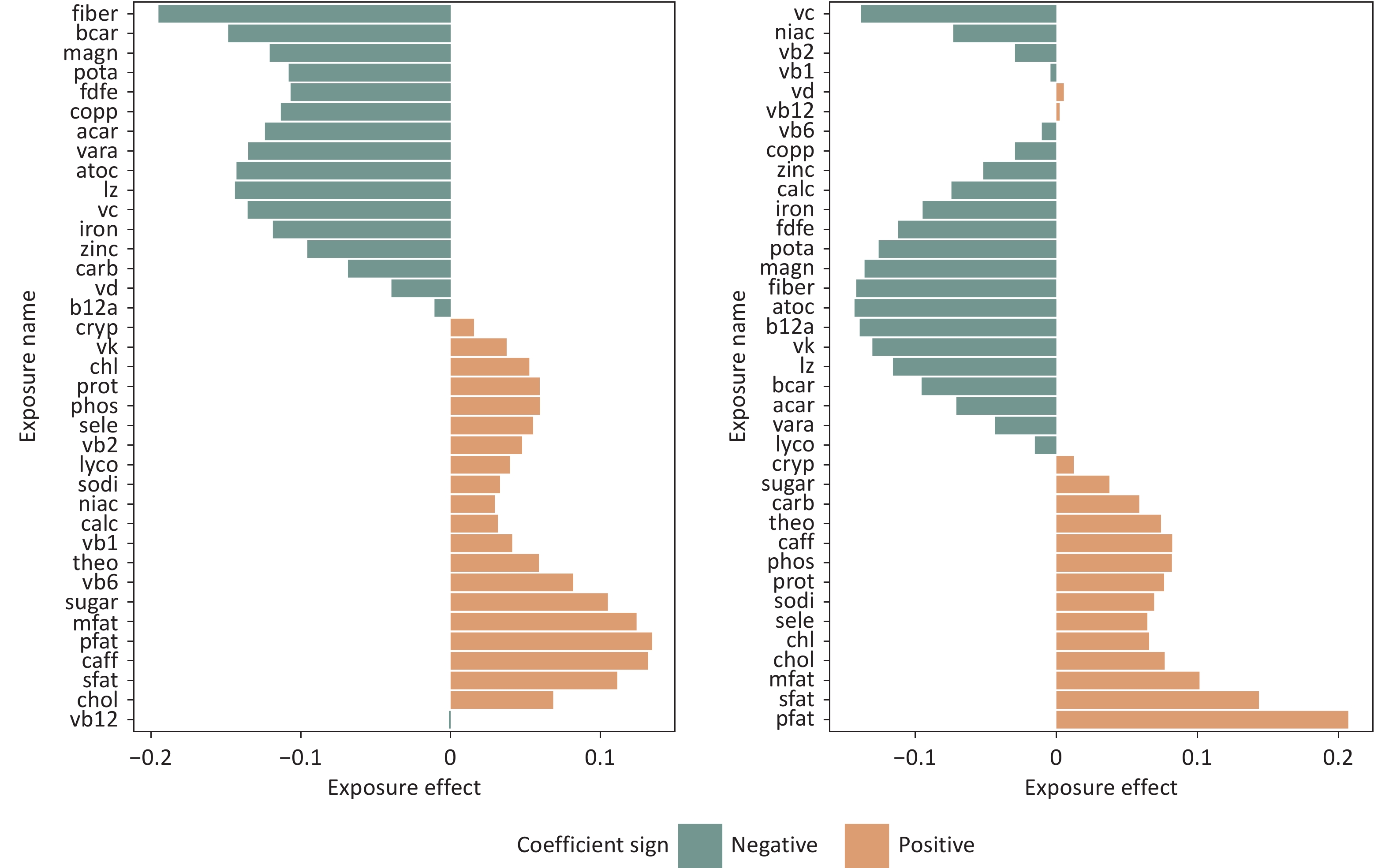
The GFLM model was applied to reanalyze data from the NHANES 2011–2016 cycles to examine and estimate the effects of 37 nutrients on BMI, while also demonstrating the relative contribution of each nutrient. Analysis of variance inflation factors (VIF) revealed correlation among the nutrients, with 9 nutrients showing high correlation (VIF > 5) and 14 showing moderate correlation (2 < VIF ≤ 5). Table 2 presents the estimated mixture effects, 95% CIs, and test results for the different exposure ordering mechanisms. After controlling for covariates, the nutrient mixture had a significant effect on BMI. Under association-based ordering, a one-quartile increase across all nutrients corresponded to a 0.246 unit decrease in BMI. Under correlation-based ordering, this effect was estimated as a 0.323-unit decrease.

Figure 8 illustrates the effect function calculated using model (3) for both ordering mechanisms. While Renzeitt’s^[10] work identified magnesium and sodium as the nutrients with the largest negative and positive contributions, respectively, the GFLM analysis suggests a more nuanced interpretation. Although these nutrients have both negative and positive effects, they are not significant contributors. Instead, their effects appear to be a part of a complex interplay with other nutrients. Figure 8 shows that fiber and fat consistently emerged as nutrients with the greatest negative and positive effects, respectively, regardless of the ordering method. This finding is consistent with those of numerous previous studies on the effects of diet on BMI^[25-27].

Figure 8.  Nutrient effect estimates under association-based and correlation-based ordering assumptions (NHANES 2011–2016).

Notably, for certain nutrients, the estimated direction of the effect differed between the two ordering mechanisms. This discrepancy is related to the GFLM estimation methodology and warrants further discussion in the subsequent sections of this paper.

The GFLM model was applied to analyze data from the NHANES 2007–2018 cycles to investigate the association between the four PFASs and gout risk while controlling for various covariates.

Analysis of the dataset revealed strong linear correlations between the four PFAS, as illustrated by the Pearson correlation coefficient matrix in Table 3. A multistep analytical approach was used to examine the relationship between PFAS exposure and gout risk. Initially, logistic regression models were used to assess the association between individual PFAS and gout after adjusting for all covariates. Subsequently, a multivariate logistic model incorporating all the four PFAS was constructed to explore their combined effects. The results of these analyses are presented in the “individual exposure analysis” section in Table 4. Both the univariate and multivariate analyses showed no significant association, with only PFOA exhibiting marginal significance in the multivariate model. However, recognizing the limitations of logistic regression in capturing the mixture effects, further analysis was conducted using both WQS and the proposed GFLM. The results are presented in the lower half of Table 4.

WQS regression analysis suggested a significant association between the joint effect of the four PFAS and gout risk (OR, 1.40; 95% CI: 1.31–1.50). In contrast, the GFLM showed no significant association. To interpret this discrepancy in the results, we noticed high positive correlations among the PFAS, as shown in Table 3, which suggests that multicollinearity may significantly influence parameter estimation in the WQS framework. Moreover, the discrepancy can be understood through simulation studies, which demonstrate that WQS tends to overestimate the mixture effects for binary outcomes. Given this tendency and the fact that GFLM’s demonstrated robust performance in the simulations, the GFLM results suggesting no significant PFAS mixture effect on gout risk may be more reliable.

In this study, we propose a novel model framework for analyzing mixture exposure data. Drawing inspiration from the FDA, we introduce the concept of fitting the exposure effects as continuous functions. This approach allows for efficient and accurate effect estimation, while fully capturing the correlations between exposures. Statistical simulations demonstrated that the proposed GFLM model exhibited a robust performance and preferable statistical power across various settings. The effect size estimates were reliable, with 95% CIs consistently encompassing the true values across all simulation scenarios. We applied the model to reanalyze the effects of 37 nutrients on BMI using the NHANES database, which yielded results that were more interpretable than those of the original study. Additionally, the application of the GFLM to the PFAS-gout dataset further demonstrated its utility in handling complex, correlated exposures. Unlike the WQS regression, which suggested a significant association between the PFAS mixture and gout risk, the GFLM showed no significant association. This discrepancy highlights GFLM’s robustness of the GFLM to multicollinearity, which is a common challenge in environmental mixture analysis.

Given the innovative integration of FDA techniques into mixture exposure analyses, it is essential to highlight the key technical considerations for practical applications. Typically, functional regression is applied when variables are functions of time or other continua; however, exposure generally lacks inherent order. To address this, our analytical framework first orders the exposures according to specific rules and then approximates the position as a continuous quantity for function fitting. The scientific basis for this approach stems from observations in time-series data, where adjacent points often exhibit the highest correlation, leading to our proposed correlation-based ordering mechanism, which arranges exposures based on the hierarchical clustering of their associations. Although the selection of basis functions is an important consideration in the FDA, our simulation results demonstrate that the GFLM maintains a robust performance across different choices of basis function numbers. We recommend starting with $ K=m/4 $ basis functions for general applications, where $ m $ is the number of exposures, with adjustments based on cross-validation results. Importantly, the validity of GFLM’s conclusions of the GFLM remained stable across different dimensionality reduction rates.

The implications of the two proposed ordering methods are notable. Although correlation-based ordering satisfies the conditions for functional regression, studies have shown that two positively associated exposures or biomarkers can have opposing effects on the outcome^28,29. This phenomenon explains why some exposures in our data analysis exhibited opposite effects under different ordering mechanisms. Therefore, we also propose an ordering based on the strength of the association with the outcomes. In practical applications, researchers should carefully consider the potential mechanisms of the exposure effects and select the most appropriate ordering method.

The choice between LRT and GT should be guided by study characteristics and research priorities. While the LRT shows slightly elevated Type I error rates but higher power when the effects are concentrated in fewer exposures, the GT maintains strict control and performs better when the effects are distributed across multiple exposures. GT is recommended when strict type-I error control is required, whereas LRT may be preferable for exploratory analyses or when higher sensitivity is acceptable.

Our study findings provide guidance for interpreting effect size estimates. In real-world scenarios, mixture exposure often includes near-zero-effect exposure. However, the functional regression fitting process may assign small pseudo-effects to these exposures to maintain the functional smoothness. The strength of the GFLM lies in identifying consistent patterns and peak effects across different ordering mechanisms rather than precisely estimating individual effects. Traditional regression approaches are appropriate for investigating specific exposure effects. When using the GFLM, we recommend focusing on effects that remain consistent across different ordering mechanisms, as these provide stronger evidence of true associations. Visualizations such as those in Figure 8 can be used to observe the relative contributions of each exposure within the mixture.

The proposed GFLM method has several advantages. It provides results that align more closely with the researchers’ expectations from statistical analyses. By leveraging the nested model framework and functional regression techniques, we calculated exact p values, mixture effect estimates, and CIs. Unlike the complex results of methods such as BKMR, these outputs are both familiar and easily interpretable. Second, the GFLM model exhibited superior computational efficiency. It is significantly faster than WQS, with computation times approximately 1/50 of the latter for sample sizes of 1000 under the simulation settings described in Section 2.2. This advantage became even more pronounced with larger sample sizes. A detailed comparison of the running times is provided in the Supplementary file.

However, GFLM has some limitations. First, its theoretical foundation requires a higher level of statistical expertise from users, including programming proficiency. Second, the functional regression approach in Model (3) lacks standardized guidelines for selecting the basis function system, number, and order, thus requiring researchers to explore these aspects independently. In our simulations and data analysis, we used a quarter of the number of exposures and employed B-spline fitting for cubic functions, although Fourier basis functions might be more appropriate in some cases, depending on the specific research needs. Finally, for exposures with weak individual and mixture effects, their estimated contributions can be sensitive to the choice of ordering mechanism, necessitating careful interpretation based on the researchers’ understanding of the problem.

In conclusion, the GFLM model presented in this study offers a theoretically sound and highly applicable method for analyzing mixture exposure. Statistical simulations and case analyses demonstrated their robustness, efficiency, and versatility. We have included R codes for the simulation and data analysis in the Appendix with the hope that this method will find widespread application in mixture exposure research, thereby advancing the field of public health.