

 下载:
下载:


-
In Poland, excessive airborne particulate matter (PM) pollution (often referred to by the mass media as PM smog phenomenon) has been occurring for decades[1]. The problem is so serious that Poland has now become the smog capital of Europe. The main source of Polish smog is the so-called municipal emission, more specifically, burning fossil fuels and biomass for residential heating. In some periods and/or selected locations, traffic emissions can be a significant source of smog[2-3]. Unlike the energy sector of most European Union (EU) countries, the Polish energy sector is almost totally dependent on coal, which is the main source of primary PM and precursors of secondary atmospheric particulates[4]. Although Poland has undergone a significant industrial transformation in the last 20 years, with a marked decrease in PM pollution, PM-related smog episodes are still frequent, especially in the southern part of the country[1-2, 5]. The phenomenon of PM smog (which can be physically felt as a noticeable burnt odor or manifests as visibility reduction) occurs under unfavourable meteorological conditions, such as atmospheric stagnation, low wind speed, and high relative humidity[6]. In Poland, smog is observed mostly in the winter season under strong ground-based temperature inversions. Despite conditions that favor pollutant dispersion, PM exceedances are sometimes caused by unusually high local emissions, such as those in densely built-up residential areas, where houses are equipped with outdated and inefficient boilers. Smog episodes can vary and include local smog, which covers small-range areas and is often associated with specific emission events[7]; regional smog, which covers medium-sized regions, like industrial districts or cities, and includes instances such as the famous Ruhr District episode in 1962[8] or the London episode in 1952[9]; and also, most interestingly, mesoscale smog, in which the impacted area is extended to metropolitan scale or even covers a whole country[10]. Results of epidemiological and clinical studies indicate that high concentrations of PM2.5 and PM10 in Poland are correlated with the total mortality rate due to respiratory and blood diseases[11-12]. More than 42, 000 premature deaths are attributable to the excessive concentrations of PM2.5[13]. Recent findings show that Polish cities struggle with increased incidences of PM-induced lung cancer (from 9.6 to 22.8 cases per 100, 000 inhabitants in cities)[14]. So far, there has been no indication of the extent to which PM concentration or its chemical properties [e.g., the content of toxic compounds, some metals, and polycyclic aromatic hydrocarbons (PAHs)] are responsible for the occurrence of lung cancer effects in the population. Although an increase in the frequency of these effects is usually hardly observable, the chronic character of exposure to those pollutants allows us to infer that PM episodes have a significant impact on human health[15]. The extent to which the incidence of smog events, especially on a large scale, increases the probability of negative health outcomes, is currently unclear. Given the lack of a threshold in PM concentration below which no cancer effects will occur, even low concentrations of PM-bound carcinogens may lead to the development of lung cancer. The purpose of this work is to answer to the following question: To what extent does the occurrence of the large-scale PM10 smog episodes in Poland elevate the concentrations of PM10-bound ambient carcinogens As, Cd, Ni, Pb, and Benzo(a)pyrene [B(a)P]?
We also aim to check whether these situations lead to an increased number of lung cancer cases in the general population. In this work, we compared the magnitude of inhalation exposure to these pollutants between three types of areas, namely, Polish cities, large urban agglomerations, and the remaining areas.
-
Our analysis was performed based on data concerning PM10 and PM10-bound As, Cd, Ni, Pb, and B(a)P concentrations, which were measured across the whole country between 2002 and 2014 under the Polish National Air Monitoring Program. The number of air monitoring stations that provide such measurements is presented in Table S1 (available at www.besjournal.com). The episodes were selected from a series of daily (24 h) PM10 concentrations registered within the mentioned period. At present, clearly defined thresholds of PM10 daily concentrations that classify a given day as a smog episode are not available[16]. Although a couple of examples are available where these thresholds were defined by appropriate statistical processing of the daily data series[17-18], none of them can be treated as a gold selection standard. Before setting the selection criteria for these episodes, each series of the PM10 concentrations from each monitoring site was directed to distribution testing by using the Shapiro-Wilk test (P = 0.05). The assumption was that if the log-normal distribution was prevailing (i.e., more than 50% of all cases), then the median value (or arbitrarily defined percentile) of the annually averaged daily concentrations could be set as a criteria of episode occurrence in a given location[10]. If, however, the distribution was mostly normal (Gaussian), then each PM10 concentration that exceeded the value of the arithmetic mean from the annually averaged daily concentrations should be treated as an episode[19]. A summary of the results from this analysis is given in Table 1. In 32% of all the tested cases, the statistical distribution of PM10 was log-normal (P < 0.05). The lack of a clear dominance of any of the tested distributions did not allow us to use the statistical method as a criterion for episode selection. Therefore, in accordance with the literature[20], the exceedance of the average daily PM10 concentration above 50 μg/m3 (the 24 h threshold value) was set as a criterion for qualifying this as an episode day. We looked for large-scale episodes only. Thus, we assumed that country-level smog occurs when the 50 μg/m3 concentration was exceeded in at least 50% of all monitoring stations at the same day. On the basis of these criteria, 348 days were selected as large-scale smog events in the 2002-2014 period. This finding means that during the 12-year period, more than 50% of all air monitoring stations in Poland registered a PM10 daily concentration of above the permissible level of 50 μg/m3 over a total of 348 days. The greatest number of such episodes occurred in 2011, with 51 episodes, and the least number of episodes occurred in 2004, with only one episode (Table 1). Assuming that the winter season in Poland lasts from November to March, 307 episodes were assigned to the winter/cold season (the heating season).
Table 1. Results of Testing the Probability Distribution of PM10 Daily (24 h) Concentrations;
Monitoring Period Total Number of Air Monitoring Stations* Number of Stations at Which the Daily PM10 Data Series Met the Criterion of Normal Distribution Number of Stations at Which the Daily PM10 Data Series Met the Criterion of Log-normal Distribution Number of Summer/Winter Spisodes Within Calendar Year Number of PM10 Episodes in Each Calendar Year 2002 17 0 9 6/7 13 2003 54 0 22 0/7 7 2004 121 0 44 0/1 1 2005 166 1 68 6/11 19 2006 163 0 59 1/23 24 2007 173 0 64 2/12 14 2008 164 0 56 2/10 12 2009 167 0 60 7/20 26 2010 150 0 35 0/43 43 2011 143 0 30 5/46 51 2012 151 0 14 2/51 53 2013 141 0 52 5/40 45 2014 158 0 53 4/36 40 Note. *All Polish air monitoring stations that provide the measurements of PM10 concentration by using automated or manual methods from http://powietrze.gios.gov.pl[ 21 ] (Supplementary materials available at www.besjournal.com).In the second part of the analysis, we prepared the database, including the average daily concentrations of PM10-bound As, Cd, Pb, Ni, and B(a)P measured in Poland between 2002-2014. This database was divided into two parts: the first part covers the days of episodes, and the second part covers the rest of the measurement period. In each part of the data, the average daily concentrations were spatially aggregated within agglomerations (cities within provinces with more than 250, 000 residents), cities within provinces and outside the agglomerations with a total population of more than 100, 000, and areas located within provinces but lying outside the cities and agglomerations (hereafter referred to as remaining areas for more details, see the Supplementary materials available at www.besjournal.com).
Annually averaged concentrations of PM10-bound As, Cd, Ni, Pb, and B(a)P were further compared with the EU air quality standards concerning human health protection, namely, EU Directive 2004/107/EC[22] and air quality recommendations[23-24]. Significant differences in the mean concentrations of metals and B(a)P between periods with and without the episodes were checked. Given that the averaged multi-annual concentration data tend to follow a normal distribution (Shapiro-Wilk test, P > 0.05), the difference between the pair of measurements (di = xwith E -xwithout E) was tested by using Student's t-test for dependent samples (P = 0.05). This difference was further used to verify the hypothesis that the average for each difference in the studied population is 0 (H0). The significance value in the Levene's test was greater than our alpha (P > 0.05). Thus, we cannot reject the null hypothesis (no difference) for the assumption of the variance homogeneity, which means that concentrations were drawn from populations with the same variance (Tables 3-5).
Table 2. Inhalation Unit Risks and Cancer Potency Factors for Risk Analysis[29]
Carcinogen Inhalation Unit Risk (µg/m3)−1 Inhalation Slope Factor (CSFi) (mg/kg×d)−1 Arsenic 3.3 × 10⁻³ 1.2 × 101 Cadmium 4.2 × 10⁻³ 1.5 × 101 Lead 1.2 × 10⁻⁵ 4.2 × 10⁻² Nickel (nickel oxide) 2.6 × 10⁻⁴ 9.1 × 10⁻¹ B(a)P 1.1 × 10⁻³ 3.9 × 100 Table 3. Average concentrations (ng/m3) of As, Cd, Pb, Ni, and B(a)P in 12 Polish agglomerations in the 2002–2014 period. The significance (t-test, P < 0.05) and variance homogeneity (Levene's test) between mean concentrations in periods with episodes versus those without episodes are shown.
Constituents AGGLOMERATIONS Levene's test P-Value paired t-test Ds. Kp Lb Ld Mp Mz Pd Pm Sl-G Sl-RJ Wp Zp Mean Std.Dev F Sig As WITH_E 2.6 3.3 1.0 2.1 1.8 0.4 0.6 1.4 2.4 2.9 1.8 1.3 1.8 0.9 0.1237 0.7283 0.00042 As WITHOUT_E 2.4 2.9 0.9 1.9 1.7 0.3 0.6 1.3 2.1 2.6 1.7 1.0 1.6 0.8 Cd WITH_E 0.6 1.1 0.5 0.9 1.4 0.7 0.7 0.4 1.1 1.0 0.7 0.7 0.8 0.3 0.1151 0.7375 0.000792 Cd WITHOUT_E 0.6 1.0 0.4 0.8 1.3 0.7 0.7 0.4 1.0 0.9 0.6 0.6 0.7 0.3 Pb WITH_E 21.7 45.0 12.5 22.5 45.0 31.9 8.4 15.8 91.4 43.0 21.2 29.9 32.2 22.1 0.0141 0.9065 0.005969 Pb WITHOUT_E 19.9 38.0 12.1 20.0 44.0 31.0 7.7 14.8 90.4 40.0 19.7 29.3 30.7 22.3 Ni WITH_E 3.6 2.6 1.7 2.3 3.1 5.2 1.2 2.6 2.3 2.0 1.2 3.4 2.6 1.1 0.0002 0.9887 0.003426 Ni WITHOUT_E 3.6 2.6 1.7 2.2 3.0 5.1 1.2 2.7 2.3 1.9 1.2 3.3 2.5 1.1 BaP WITH_E 3.9 3.4 0.5 7.9 4.3 1.7 2.1 1.8 7.9 12.3 3.2 1.6 4.1 1.5 0.8578 0.3643 0.025991 BaP WITHOUT_E 3.0 3.4 0.5 6.8 2.6 1.4 1.9 1.4 6.2 8.5 3.2 1.6 3.5 2.5 Note. The significance (t-test, P < 0.05) and variance homogeneity (Levene’s test) between mean concentrations in periods with episodes versus those without episodes are shown. Ds-Wroctawska Kp-Bydgoska, Lb-Lubelska, Ld-todzka, Mp-Krakowska, Mz-Warszawska, Pd–Białostocka, Pm–Trójmiejska, Sl-G–Górnośląska, Sl-RJ–Rybnicko-Jastrzębska, Wp–Poznańska, Zp–Szczecińska. Table 4. Average concentrations (ng/m3) of As, Cd, Pb, Ni, and B(a)P in the 16 remaining (other than cities and agglomerations) areas of Poland in the 2002-2014 period.
Constituents REMAINING AREAS Levene's test P-Value paired t-test Ds. Kp Lb Lu Ld Mp Mz Op Pk Pd Pm Sl Sk Wm Wp Zp Mean Std Dev F Sig As WITH_E 3.8 1.9 0.4 3.4 2.0 1.5 0.6 2.3 1.4 0.3 1.4 3.0 - 1.1 2.3 0.8 1.7 1.1 0.1237 0.7283 0.001421 As WITHOUT_E 3.6 1.8 0.4 3.3 1.8 1.4 0.6 2.4 1.2 0.3 1.4 2.8 - 1.0 2.1 0.7 1.6 1.0 Cd WITH_E 1.0 1.0 0.7 0.6 0.6 1.1 0.6 0.5 1.1 - 0.4 1.4 1.3 0.2 0.8 0.5 0.8 0.3 0.1151 0.7375 0.000003 Cd WITHOUT_E 0.9 0.9 0.6 0.6 0.6 1.0 0.5 0.4 1.0 - 0.4 1.3 1.3 0.2 0.8 0.5 0.7 0.3 Pb WITH_E 40.0 20.7 8.3 24.3 21.0 31.6 20.7 20.6 27.3 13.0 18.4 58.7 - 5.4 20.7 17.4 23.1 13 0.0141 0.9065 0.000054 Pb WITHOUT_E 39.0 20.2 7.8 21.9 19.0 28.8 19.9 19.9 25.4 12.8 17.3 57.0 - 4.9 18.6 16.7 22.0 12.6 Ni WITH_E 3.8 1.6 2.0 2.8 2.1 3.7 2.4 2.4 1.4 0.5 4.1 5.0 3.8 0.7 3.1 3.4 2.6 1.1 0.0002 0.9887 0.079302 Ni WITHOUT_E 3.9 1.5 2.0 2.8 2.0 3.7 2.4 2.2 1.4 0.5 4.1 3.8 3.3 0.6 3.1 3.3 2.6 1.2 BaP WITH_E 4.8 3.2 2.6 4.5 9.8 7.7 3.6 4.6 5.5 1.8 5.1 7.9 5.2 0.6 2.5 3.4 4.1 2.3 0.8578 0.3643 0.003419 BaP WITHOUT_E 4.0 3.1 2.4 3.3 7.6 4.2 2.6 2.1 3.6 1.8 3.4 6.9 4.3 2.1 2.5 2.7 4.0 1.8 Note. The significance (t-test, P < 0.05) and variance homogeneity (Levene's test) between mean concentrations in periods with episodes versus those without episodes are shown. Ds.–Dolnośląska, Kp–Kujawsko-Pomorska, Lb–Lubelska, Lu–Lubuska, Ld-Łódzka, Mp–Krakowska, Mz-Mazowiecka, Op–Opolska, Pk–Podkarpacka, Pd–Podlska, Pm–Pomorska, Sl–Śląska, Sk–Świętokrzyska, Wm–Warmińsko-Mazurska, Wp–Wielkopolska, Zp–Zachodniopomorska. The lack of data "-". Table 5. Average (ng/m3) concentrations of As, Cd, Pb, Ni, and B(a)P in 18 Polish cities in the 2002-2014 period.
Constituents CITIES Levene's test P-Value paired t-test Ds. Leg Ds. Walbrz Kp Toru Kp Wlocl Lu Gorz Lu Ziel Mp Tar Mz Plock Mz Radom Op Opole Pk Rzesz Sl Biel Sl Czesto Sk Kiel Wm Elb Wm Olszty Wp Kalisz Zp Kosz Mean Std Dev F Sig As WITH_E 8.3 2.2 1.3 1.0 1.4 3.7 1.2 0.7 0.4 2.5 1.5 2.2 3.0 1.9 1.7 1.4 2.2 0.6 2.1 1.8 0.0064 0.9367 0.000108 As WITHOUT_E 8.0 2.2 1.2 0.9 1.4 3.7 1.1 0.7 0.3 2.4 1.3 2.0 2.7 1.6 1.7 1.3 2.0 0.5 1.9 1.7 Cd WITH_E 1.2 0.8 1.2 1.4 0.5 0.5 1.6 0.8 0.4 1.8 0.8 0.7 1.1 1.3 0.2 0.2 0.6 0.5 0.9 0.5 0.0568 0.8129 0.000549 Cd WITHOUT_E 1.1 0.7 1.2 1.4 0.5 0.4 1.6 0.8 0.4 1.8 0.7 0.6 1.0 1.1 0.2 0.2 0.5 0.4 0.8 0.5 Pb WITH_E 144.0 25.8 12.4 27.5 24.6 25.7 22.9 27.1 18.7 38.5 23.6 25.4 37.0 34.7 6.9 4.5 15.6 14.4 29.4 30.1 0.0009 0.9760 0.000001 Pb WITHOUT_E 142.0 24.1 11.6 25.7 24.0 24.8 21.8 26.6 16.1 35.8 19.7 22.2 35.0 32.2 6.0 4.0 13.4 13.4 27.7 30.0 Ni WITH_E 3.3 6.4 1.9 2.7 3.4 2.5 2.1 2.7 1.3 5.9 1.1 1.9 2.5 2.2 1.0 0.7 1.9 3.0 2.6 1.5 0.0176 0.8949 0.021427 Ni WITHOUT_E 2.7 6.4 1.8 2.7 3.3 2.4 2.1 2.7 1.3 5.6 1.1 1.9 2.5 2.1 1.0 0.7 1.8 3.0 2.5 1.5 BaP WITH_E 6.6 5.0 2.3 2.3 3.9 1.9 3.5 4.7 4.3 7.6 2.7 5.3 3.1 5.8 2.9 1.3 3.5 3.2 3.9 1.7 0.8595 0.3603 0.000958 BaP WITHOUT_E 5.2 4.7 1.9 2.3 2.1 1.6 3.5 4.1 3.8 6.4 2.7 3.1 2.9 4.7 2.9 1.1 3.5 2.4 3.3 1.4 Note. The significance (t-test, P < 0.05) and variance homogeneity (Levene's test) between mean concentrations in periods with episodes versus those without episodes are shown. DSLeg-Legnica, DsWalbrz-Wałbrzych, KpToru-Toruń, KpWlocl-Włocławek, LuGorz-Gorzów, LuZiel-Zielona Góra, MpTar-Tarnów, MzPlock-Płock, MzRadom-Radom, OpOpole-Opole, PkRzesz-Rzeszów, SlBiel-Bielsko-Biała, SlCzesto-Częstochowa, SkKiel-Kielce, WmElb-Elbląg, WmOlszty-Olsztyn, Wp-Kalisz-Kalisz, ZpKosz-Koszalin. -
Lung cancer risk that resulted from the exposure to PM10-bound As, Cd, Pb, Ni, and B(a)P was assessed using the deterministic approach[25] according to the US EPA[26] reference methodology. The analysis was performed for periods with and without episodes separately for agglomerations, cities, and remaining areas. The exposure scenario includes the lifetime inhalation exposure of a hypothetical adult Polish resident (without division between male or female).
-
The active dose of inhaled carcinogens, namely, metals and B(a)P, was assumed to be equal to the airborne concentration and calculated following Equation 1:
$$ {E_i} = {C_i} \times IR $$ (1) Where Ei – daily exposure level to ith carcinogen in the adult age group (ng/d), Ci– concentration of ith carcinogen in the air (ng/m3), IR-inhalation rate among adults; the 95th percentile of IR for people 31 to 41 years old is 21.4 m3/day, following US EPA[27].
-
The possibility of additional lung cancer risk was estimated using Incremental Lifetime Cancer Risk (ILCR)[28]. ILCR represents the probability of an individual to develop cancer over his or her lifetime from exposure to PM10-bound metals and B(a)P (for example, 1:100, 000 indicates one case of cancer in a population of 100, 000). The ILCR value was calculated on the basis of Equation 2, and CSF values for carcinogenic pollutants were used in accordance with the Office of Environmental Health Hazard Assessment database (Table 2)[29]. The risk to humans was calculated independently for each pollutant and then summarized. The cumulative lifetime cancer risk as a result of exposure to multiple carcinogens is obtained. This cumulative ICLR was compared with the threshold value. The level of acceptable cancer risk for regulatory purposes is considered within the range of 1 × 10⁻⁶ to 1 × 10⁻⁴[30].
$$ ILCR = \frac{{{E_i} \times EF \times ED \times \left( {CS{F_i}} \right)}}{{BW \times AT}} \times cf $$ (2) Where ILCR– incremental lifetime cancer risk resulting from a specific dose of carcinogen, Ei– daily exposure level to ith carcinogen in the adult age group (ng/d), CSFi– slope factor for ith carcinogen (kg × d/mg), EF– exposure frequency (day/year)[31], ED– exposure duration (year) (human lifespan: 70 years), AT– average time for carcinogens AT = 70 (year) x 365 (day/year)[32], BW– body weight (70 kg)[27], cf– conversion factor (10−6) (ng/mg).
To check whether PM10 episodes significantly increase the overall health risk from PM10-related metals and B(a)P, t-test for paired data was performed in accordance with the scheme presented in the section 'Selection of Episodes'. This approach involves comparing the P-value with the significance level (P = 0.05) and rejecting the null hypothesis when the P-value is less than the significance level.
-
Tables 3-5 present the average PM10-bound As, Cd, Pb, Ni, and B(a)P concentrations in Polish cities, agglomerations, and remaining areas divided into periods with and without episodes. Table S2 (available at www.besjournal.com) shows the significance of the differences in concentration data between those groups. The mass concentrations of PM10-bound metals indicate that in most cases, their concentrations were within acceptable standards (Tables 3-5), while the B(a)P threshold value (1 ng/m3[22]) was exceeded in almost every part of the country. The greatest air pollution by B(a)P in periods with and without episodes occurs in the heart of Śląskie Province, specifically in the Rybnicko-Jastrzębska agglomeration (12.3 ng/m3) (Table 3), which is considered the cradle of Polish mining. In the Łódzka agglomeration, which also lies in the European air pollution hotspot area[33], the B(a)P concentrations were slightly lower (7.9 ng/m3) than those in the Górnośląska agglomeration, but they also far exceeded the threshold value. In areas located outside the cities and agglomerations (the remaining areas), the highest concentrations of B(a)P were recorded in Łódzka area (9.8 ng/m3), Krakowska (7.72 ng/m3), and Śląska (7.92 ng/m3) (Table 4). Much lower concentrations were found in the northern part of Poland, specifically the areas within Warmińsko-Mazurskie and Podlaskie provinces) (Table 3) with average multi-year concentrations of 0.62 and 1.79 ng/m3, respectively.
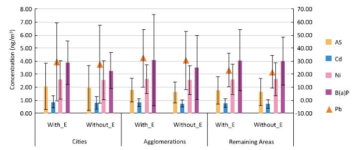
Regardless of the area type, Pb had the highest mass concentrations among metals and was followed by Ni, As, and Cd. The average Pb concentrations in cities, agglomerations, and remaining areas during 2002-2014, including episode occurrence, were 29.4, 32.3, and 23.2 ng/m3, respectively, and were slightly lower and estimated at 27.6, 30.6, and 22 ng/m3, respectively, after excluding the episodes. Higher mean concentrations of As, Cd, and Ni in 2002-2014 were also observed in the dataset that includes episodes. The highest concentrations of As and Cd was recorded in the cities– (8.3 ng/m3-Ds Leg.) and (1.8 ng/m3 Op.), respectively (Table 5). The highest Ni concentration recorded in the agglomerations was 2.61 ng/m3 (Table 3). The highest multi-year average concentrations of As and Pb occurred in Legnica with 8.32 and 144 ng/m3, respectively, which is a direct result of their release from the Legnica copper plant. In terms of Pb concentrations, the Górnośląska agglomeration ranked second among all agglomerations, with an average concentration of 91.4 ng/m3. The source of metals in the Górnośląska and Rybnicko-Jastrzębska agglomerations, as in the case of Legnica, is the emissions from industrial processes and combustion of fuels in household ovens and car engines[34-36]. Industrialization and metallurgical processes have left a mark on air quality and the destruction of natural resources, especially in the southern regions of the country, which are richly endowed with minerals and coal deposits[37]. Therefore, the difference between the regional levels of metal concentrations generally decreases from the northeast to the southwest of Poland. The spatial distribution of metals (Figure 1) indicates that area type does not greatly influence the concentration levels of PM10-bound As, Cd, Pb, and Ni.
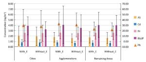
Figure 1. Average PM10-bound metals and B(a)P ambient concentrations in Poland over the 2002-2014 period [including episode (with_E) and without episode occurrence (without_E)]. The bars denote the average mean concentration, while the whiskers denote standard deviation.
In terms of area type, the PM10-bound metal concentrations change slightly in the following descending order: cities > agglomerations > remaining areas (As); cities > agglomerations > remaining areas (Cd); agglomerations > cities > remaining areas (Pb); and remaining areas > agglomerations > cities (Ni). Unlike the metal concentrations, the mean B(a)P concentrations throughout the 2002-2014 period were significantly higher in remaining areas compared with those in cities or agglomerations (Tables 3-5), which is a direct result of spatial differences in emission from residential combustion sources.
-
Figures 2-4 show a comparison of the inhalation lifetime cancer risk calculated in the scenario included the episode occurrence and assumed their absence according to administrative division. These figures present the spatial distribution of the cumulative lifetime cancer risk among considered cities, agglomerations, and remaining areas. Figure 5 presents the total cancer risk averaged within these differently polluted locations.
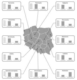
Figure 2. Cumulative lifetime lung cancer risk (ILCR) resulting from exposure to PM-bound As, Cd, Pb, and Ni in Polish agglomerations presented in two datasets, namely, including (ILCR With_Episodes) and excluding PM10 episodes (ILCR Without_Episodes). E-05, × 10-5; E-06, × 10-6.
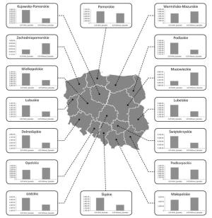
Figure 3. Cumulative lifetime lung cancer risk (ILCR) resulting from exposure to PM-bound As, Cd, Pb, and Ni within Polish provinces but lying outside the agglomerations and cities (referred to as 'remaining areas' in this work) presented in two datasets, namely, including (ILCR With_Episodes) and excluding PM10 episodes (ILCR Without_Episodes). E-05, × 10-5; E-06, × 10-6.
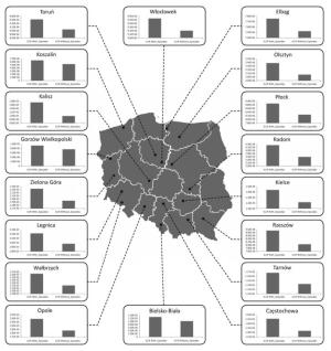
Figure 4. Cumulative lifetime lung cancer risk (ILCR) resulting from exposure to PM-bound As, Cd, Pb, and Ni in Polish cities (with more than 100, 000 residents) presented in two datasets, namely, including (ILCR With_Episodes) and excluding PM10 episodes (ILCR Without_Episodes). E-05, × 10-5; E-06, × 10-6.
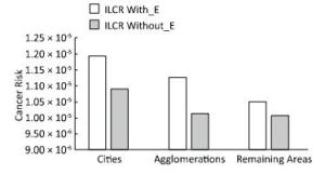
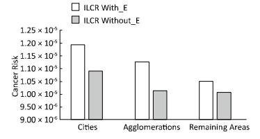
Figure 5. Cumulative lifetime lung cancer risk (ILCR) resulting from exposure to PM-bound As, Cd, Pb, and Ni in Poland presented in two datasets, namely, including (ILCR With_E) and excluding PM10 episodes (ILCR Without_E).
The cumulative lung cancer risk, as averaged between cities, agglomerations, and remaining areas in the dataset that includes episodes, was 1.13 × 10⁻⁵, whereas it was 1.04 × 10⁻⁵ in the dataset that excludes the influence of the episodes and did not exceed the acceptable risk (1 × 10⁻⁴). Among all the considered cities, the highest cancer risk was found in Częstochowa, Kielce, Legnica, Opole, Wałbrzych, and Zielona Góra both in the periods with and without the episodes. The averaged 'ILCR With_Episodes' value within those locations was 1.8 × 10⁻⁵, while it was one order of magnitude lower and estimated at 1 × 10⁻⁶ among the cities lying in the north (i.e., close to the Baltic Sea), such as Elbląg, Olsztyn, and Włocławek. Among agglomerations, the highest risk value was found in Górnośląska and Rybnicko-Jastrzębska areas with 'ILCRWith_Episodes' values equal to 1.74 × 10⁻⁵ and 2.15 × 10⁻⁵, respectively. An interesting exception can be found in the remaining areas in Zachodniopomorskie and Mazowieckie provinces (Figure 3), where the number of cancer occurrences in the periods with episodes is lower than that in the periods excluding the episodes. However, this observation is expected because these provinces are among the wealthiest and most economically developed areas of Poland, with the highest GDP per capita and whose commercial energy sector (even in the rural areas) is based on ecological solutions. Therefore, the rural energy-related PM emissions in these areas is much lower than that in the rest of the country.
When averaging ILCR within all cities, the number of lung cancer cases in those areas was approximately 9% higher than the risk found within the remaining areas (regardless of episode occurrence) (Figure 5). This observation is in good agreement with the popular opinion that urban dwellers are at a higher health risk than citizens living in rural areas or areas located some distance from the agglomerations. The observed dependencies are, however, burdened by fluctuations in the availability of the monitoring data among different provinces and monitoring station types (Table S1, available at www.besjournal.com). In fact, Polish cities and agglomerations are more densely covered by air monitoring stations than other areas within the country.
-
Interestingly, while looking at the dataset in Tables 3-5, we can observe that over the past 12 years, metal concentrations were uniformly distributed between agglomerations, cities, and the remaining areas. This situation results from the fact that the energy-related emissions of PM and PM-bound metals in Poland have not undergone any significant changes over the last years. Taking into account the source category, the highest share of metal emission loadings into the atmosphere is attributable to the 1.A.1 Public Power and Industrial Comb sector according to the Selected Nomenclature for Sources of Air Pollution (SNAP97)[38]. The major emission of As, Cd, and Pb originates from 'combustion in industrial processes' (48%, 56%, and 49% of the total emission rate, respectively), and in the case of Ni, the emissions originate from 'combustion processes outside industry' (54% of the total national emission)[39]. Iron and non-ferrous metallurgy also have a significant share in the amount of the national emission of these pollutants[39-40].
Regardless of location, in almost each case, a statistically significant difference was found in metals and B(a)P concentrations between periods with and without episodes (t-test, P < 0.05) (Table S2, available at www.besjournal.com). The only exception was the lack of this relevance in the case of Ni concentrations within the remaining areas. The dependencies that we found are not surprising because PM10 episodes greatly add to the total emission load of PM pollution. In Poland, where the dominant source of PM emission into the atmosphere is burning fossil fuels in the municipal and residential sectors (57% of the PM10 fraction is produced by the combustion of solid fuels, mainly lignite and coal[40]), the PM10 concentrations are correlated mostly with the concentrations of soot and SO2. Meanwhile, metals and B(a)P in atmospheric air are primarily associated with fine particles with an aerodynamic diameter of less than 2.5 μm[41]. Stronger or more significant differences in the concentrations of metals and B(a)P between the episode and non-episode periods would be observable for PM2.5-bound compounds, especially in the residential areas that tend to be heated with wood and coal, where toxic metals are mainly bound to fine and accumulation particles[42]. Another situation of concern is high-traffic areas, where resuspension of road and soil dust greatly adds to the observed loadings of PM coarse particles[43].
The influence of smog episodes on the levels of PM10 and PM2.5-bound metals was investigated in the course of studies conducted by[2] at the crossroads and urban background site in Zabrze (in southern Poland). During the episodes, the concentrations of metals associated with PM10 increased at the roadside compared with that in the background by approximately 10 times (one order), while PM2.5-bound metals showed two to three times elevated concentrations [except Fe (five times)] and Cr (no increase)]. Other studies conducted in Krakow (also in southern Poland) found that during the temperature inversion episodes, the concentrations of PM10-bound B(a)P were 200-400 times higher than the EU target value of 1 ng/m3[44]. This finding proves that air pollution by B(a)P is one of the major environmental problems in Poland and is especially marked in the southern parts of Poland, that is, the extensively industrialized and highly polluted Śląskie coal basin[34-37, 45]. Many researchers state that local-scale air pollution episodes are much more evident than large-scale events (e.g., the whole country), where different confounding factors such as meteorological conditions can blur their occurrence[46]. This issue is the reason the Polish Institute for Environmental Protection-National Research Institute suggested that PM episodes should be analyzed at different range levels, from regional to transboundary[18].
Our calculations indicate a significant difference in the total risk between smog and non-smog periods among cities and agglomerations (t-test, P < 0.05) (Table S3 available at www.besjournal.comand Figure 5). This observation is in good agreement with the epidemiological data that showed positive associations between urban PM pollution and respiratory outcomes, such as hospital admissions for lower respiratory tract infection, chronic obstructive pulmonary disease, or asthma[47-51]. With regard to the question of the relationship between the number of lung cancer occurrences and the region type, Poland is exposed to concentrations of PM-bound As, Cd, Ni, Pb, and B(a)P that are typically found in the agglomerations and big cities, which are at greater risk compared with the remaining areas (Figure 5). This result is the sum of the risks posed by exposure to all metals and B(a)P. The magnitude of carcinogenic potency factors was higher for Cd and As than that for B(a)P (Table 2), which shifts the risk toward areas that are characterized by the highest concentrations of those elements, that is, cities and agglomerations (Figures 2-3). When looking at the concentration data (Tables 3-5), in the case of B(a)P, the greatest cancer risk will occur in the remaining areas outside the urban sites, whereas in the case of metals, more noticeable effects will occur in cities and agglomerations. Different emission inventories indicate that the less densely populated and less wealthy areas of Poland are more affected by B(a)P than the big cities. Unlike cities or agglomerations that are supplied with heat and hot water by the district heating system, most Polish suburbs and villages are heated by boilers or outdated ovens that emit excessive amounts of air pollutants, including B(a)P[42].
The link between geographical differences in air pollution and mortality/morbidity rates of lung cancer must be sought with extreme caution because the observed dependencies are a cumulative derivative of variances in society, poverty, economy, and national policies, which are often imbalanced between urban and rural areas[52]. Despite good evidence that ambient air pollution increases the risk of lung cancer not only in Poland but also around the world, we must remember that simple risk calculations, such as those presented in this study, cannot be the basis for making an inference about the existence of such a relationship. They only provide an answer to the question concerning the magnitude of exposure to a few atmospheric pollutants.
-
A significant contribution of this work is that it investigates and presents the exposure and inhalation risk related to most toxic metals and B(a)P on the basis of existing monitoring data. Moreover, this work determines the extent to which Polish episodes of excessive PM10 concentrations add to this exposure. This approach provides an important input to the discussion regarding the additive effect of the smog effect to human exposure, and it helps quantify the spatially diverse estimations of environmentally related cancer. The latest reports of Lung Cancer Research Fund International indicate that lung cancer incidences in Poland at an age-standardized rate per 100, 000 (world) averaged for males and females is 38 (WHO Cancer Today Database[53]). This result puts Poland in ninth place among countries in this category and indicates the need for further studies concerning the carcinogenic potential of air pollution, with a special emphasis on the long-term health effects of extremely high PM pollution. Our results clearly demonstrate that the occurrence of elevated PM10 concentrations in Poland on a large scale significantly increases the concentration level of carcinogenic compounds such as As, Cd, Ni, Pb, and B(a)P. This finding is a result of the significant environmental impact of PM concentration exceedances, as reflected by an increase in the concentrations of PM-bound metals and B(a)P, which constitute only a trace amount of the total PM10 mass. Our results prove that the Polish episodes of high PM10 concentrations, although predominantly local, can contribute significantly to country-level PM pollution. This finding also means that both the occurrence of smog episodes and a search for their relationships with health effects should be considered not only on a local scale but also on the country level. However, finding and demonstrating the correlations between local PM episodes and long-term health effects outside the country borders are considerable challenges. Therefore, further research should be directed to elucidate the prospects for attributing lung cancer mortality to the ambient air quality in Poland, with a special emphasis on addressing the health effects of geographical differences in the frequency and magnitude of PM10 concentration exceedances.
-
In Poland air pollution assessment is provided in 46 zones. The following zones include:
12 agglomerations: Wrocławska (DsWrocWie; DsWrocWybCon; DsWrocOrzech); Bydgoska (KpBydWarszaw; KpBydPlPozna; KpBydgUjejskiego; KpBydgWPola); Lubelska (LbLublin_Krasn; LbLubObywate; LbLubSliwins); Łódzka (LdLodzCzerni; LdLodzLegion; LdLodzRudzka; LdLodzWIOSARubinst; LdPabiKilins), Krakowska (MpKrakBulwar; MpKrakowWIOSPrad6115; MpKrakBujaka); Warszawska (MzWarAKrzywWSSE; MzWarAlNiepo; MzWarszZelazWSSE; MzWarZeganWSSE; MzWarszBorKomWSSE; MzWarAKrzywo; MzWarTolstoj); Białostocka (PdBialWaszyn); Trójmiejska (Pm.01w.01m; Pm.00.s237m; PmGdaGleboka; PmGdaLecz08m; PmGdyJozBema); Górnośląska (SlDabro1000L; SlKatoKossut; SlZabSkloCur); Rybnicko-Jastrzębska (SlRybniBorki; SlZorySikors); Poznańska (WpPoznanPM10szpital; WpPoznChwial); Szczecińska (ZpSzczecinWSSE; ZpSzczPils02; ZpSzczAndr01)
18 cities with the number of residents above 100 000: Legnica (DsLegAlRzecz); Wałbrzych (DsWalbrzWyso); Toruń (KpToruDziewu; KpTorunSzpMiejski); Włocławek (KpWloclOkrze; KpWloclLady); Gorzów Wielkopolski (LuGorzPilsud; LuGorzKosGdy); Tarnów (MpTarnowWIOSSoli6303; MpTarBitStud); Płock (MzPlockKolegWSSE; MzPlocKroJad); Radom (MzRadomCzWSSE; MzRad25Czerw); Opole (OpOpole246; OpOpoleOsAKr); Rzeszów (PkRzeszWIOSSzop; PkRzeszRejta); Kalisz (WpKaliszPM10; WpKaliSawick); Zielona Góra (LuZielKrotka); Bielsko-Biała (SlBielKossak); Częstochowa (SlCzestoBacz); Kielce (SkKielKusoci; SkKielJagiel); Elbląg (WmElbBazynsk); Olsztyn (WmOlsztyWSSE_Zolnier; WmOlsPuszkin); Koszalin (ZpKoszalinWSSE; ZpKoszSpasow)
16 remaining areas located within provinces but lying outside the agglomerations and cities: Dolnośląskie (DsCzerStraza; DsDzialoszyn; DsJelw05; DsPolKasztan; DsZgorBohGet; DsSzczKopPM; DsOlawZolnAK; DsOsieczow21; DsNowRudSreb; DsSzczaKolej; DsJelGorSoko; DsOlawZolnAK; DsGlogWiStwo); Kujawsko-pomorskie (KpCiechTezni; KpGrudzIkara; KpInowrSolan; KpNaklSkargi; KpWabrzstmob; KpDAFGolub; KpSepolno; KpDAFChelmza; KpDAFRadzyn; KpZielBoryTu; KpGrudSienki; KpKoniczynka; KpTuchPiast); Lubelskie (LbBiaPodOrze; LbChelJagiel; LbKrasKoszar; LbLeczna1000Lecia; LbRadzPodSit; LbRejowiecFabrWIOS; LbZamoHrubie; LbTomaszowLubWIOS); Lubuskie (LuWsKaziWiel; LuZaryWIOS_MAN; LuSulecDudka; LuZarySzyman); Łódzkie (LdKutnoWIOSMWilcza; LdOpocPlKosc; LdPioTrSienk; LdBrzeReform; LdRadomsRoln; LdRawaNiepod; LdSierGrunwa; LdSkiernWIOSMJagiell; LdToMaSwAnto; LdZduWoKrole; LdOpocPlKosc; LdWieluPOW12; LdLowiczSien; LdPioTrKraPr; LdSkierKonop); Małopolskie (MpTrzebiWIOSPils0303; MpSkawOsOgro; MpBochniWSSEKons0105; MpChrzanWSSEGrzy0301; MpNiepo3Maja; MpNoTargWSSESzaf1102; MpNSaczWSSETarn6202; MpProszWIOSKrol1404; MpWadowiWIOSPSka1805; MpBochniWSSEKons0105; MpGorlKrasin; MpTuchChopin; MpNoSaczNadb; MpNSaczWIOSPija6204; MpZakopaSien; MpBochKonfed; MpSuchaBWIOSHand1512; MpTrzebOsZWM; MpBrzeskWIOSWiej0202; MpDabrowWIOSZare0401; MpMiechoWIOSKono0802; MpNowyTaWIOSPows1114; MpOswiecWIOSSnia1302; MpRabkaWIOSChop1113; MpSuchaBWIOSHand1512; MpBukowKolejMOB; MpKetyWyspiaMOB; MpLimanoBoleMOB; MpMysleRynekMOB; MpSlomWolnosMOB; MpSzczawJanaMOB); Mazowieckie (MzOstMazSikorWSSE; MzCiechStrazacka; MzLegZegrzyn; MzNowDwChemWSSE; MzOstrolTargowa; MzOtwockBrzozWSSE; MzPiaseczDworWSSE; MzPruszKraszeWSSE; MzSochPlocWSSE; MzTluszczJKiel MzGranicaKPN; MzMlawOrdona; MzPiasPulask; MzOtwoBrzozo; MzSiedKonars; MzOstroHalle); Opolskie (OpGlubKochan; OpNamys2pyl; OpOlesno3pyl; OpKluczMicki; OpKKozBSmial; OpNysaRodzie; OpZdziePiast); Podkarpackie (PkPrzemWIOSPDom; PkJasloWIOSFlor2; PkMielZaStre; PkNiskoSzkla; PkJarosWIOSJanPawII; PkPrzemyslWIOSMick; PkJasloSikor; PkJarosPruch; PkPrzemGrunw; PkSanoSadowa; PkTarnDabrow; PkDebiGrottg); Podlaskie (PdSuwPulaski); Pomorskie (Pm.06.s712m; Pm.63.s079m; Pm.63.wDSMm; Pm14TCZEw06m; PmWejhPlWejh; PmWladywHallera; Pm.aw07m; PmKosTargo12; PmSlupKniazi; PmSlupOrzesz; PmKwiSportow; PmLebMalcz16; PmLinieKos17; PmMalMicki15; PmGac); Śląskie (SlZywieKoper; SlLublPiasko; SlZawSkloCur; SlRacibRaci_studz; SlCieszCies_dojaz; SlGodGliniki; SlKnurJedNar; SlMyszMiedzi; SlWodziWodz_bogum; SlPszczBoged; SlTarnoLitew; SlGodGliniki); Świętokrzyskie (SkBuskRokosz; SkStaraZlota); Warmińsko-mazurskie (WmDzialdWSSE_Biedraw; WmPuszczaBor; WmGizyckWIOS_Wodoc; WmNiTraugutt; WmIlawAnders); Wielkopolskie (WpKoniWyszyn; WpPilaKusoci; WpLeszno411000; WpGnieznoPM10; WpOstWieWyso; WpGniePaczko; WpLeszKiepur; WpWagrowLipo); Zachodniopomorskie (ZpSwinoujscieWSSE; ZpSzcSzczecinekPSSE; ZpWiduBulRyb; ZpSzczec1Maj; ZpSzcSzczecinek009; ZpMyslZaBram; ZpSzczecPrze).
Table S1. Summary Presenting the Number of Polish Air Monitoring Stations Conducting Measurements of As, Cd, Pb, Ni and B(a)P Concentrations by Type of the Station.
Year Vovoideship Urban background Rural Sub-urban Traffic Industrial As Cd Pb Ni B(a)P As Cd Pb Ni B(a)P As Cd Pb Ni B(a)P As Cd Pb Ni B(a)P As Cd Pb Ni B(a)P 2002 DS 1 1 1 1 1 1 2003 1 3 3 3 1 1 1 1 1 2 1 1 2 1 1 2004 2 6 7 6 2 2 2 2 2 2 1 1 3 1 1 2005 3 10 14 11 3 2 2 2 2 2 1 1 1 1 1 4 1 1 2006 3 12 16 12 3 2 2 2 2 2 1 1 1 1 1 3 1 1 2007 5 14 18 14 5 1 1 1 1 1 1 1 1 1 1 1 3 1 1 2008 5 12 16 12 4 2 2 2 2 2 1 1 1 1 1 1 5 1 1 2009 6 14 14 10 5 1 1 1 1 1 1 5 1 2010 6 6 5 3 6 2 3 2 2 2 1 1 1 5 1 1 2011 6 9 6 6 1 2 1 2 2 1 1 1 1 1 1 4 1 1 2012 8 8 8 8 8 2 2 2 2 2 1 1 1 1 1 1 2013 9 9 9 9 6 2 2 2 2 1 1 1 1 2014 10 10 10 10 11 1 1 1 1 1 1 2002 KP 1 2003 1 2004 1 2 2005 1 1 1 1 2006 2 1 2 1 1 2 2007 1 1 1 1 1 1 1 1 1 1 1 2008 9 8 10 9 1 1 1 1 1 2009 1 1 3 2 1 1 1 1 1 2 2 2 2010 7 8 9 7 1 1 1 1 1 1 1 1 1 1 1 1 2011 3 3 3 2 2 2 2 2 1 2 2 2 2 1 1 2 1 2 2012 4 4 4 3 2 2 2 2 1 2 2 2 2 1 2 2 2 2 2013 3 3 3 4 2 2 2 2 1 3 3 3 2 1 2 2 2 2 2014 3 3 3 3 3 2 2 2 2 2 2 2 2 2 2 2 2 2 2 2 2002 LB 1 2003 1 1 2004 1 2 1 1 1 1 2005 1 1 1 1 1 1 1 2006 3 1 2007 2008 2009 3 5 4 1 2 2 2 2010 2 2 2 2 1 2011 1 1 1 1 2012 1 1 1 1 1 2013 2 2 2 2 1 2014 2 2 2 2 3 2 2002 LU 2003 2004 2005 2006 2007 2008 3 2009 1 2010 1 3 2 1 2011 3 3 3 1 2012 4 4 4 1 2013 5 5 5 1 2014 6 6 6 6 2002 LD 2003 2004 3 2005 3 3 2006 3 3 2007 3 3 2008 3 3 2009 4 5 1 2010 6 6 1 2011 5 6 2012 13 13 1 2013 11 11 1 2014 14 14 14 2002 MP 2003 2004 1 1 1 1 2005 2006 1 2007 2 2 1 2008 9 9 9 9 1 1 1 2009 11 10 10 11 1 2010 9 10 10 10 1 1 1 1 2011 5 6 5 5 1 1 1 1 2012 5 5 5 5 1 1 1 1 2013 4 4 4 4 1 1 1 1 2014 5 5 5 5 18 1 1 1 1 2002 MZ 1 2003 1 3 1 1 1 2004 3 3 3 3 1 1 1 1 2005 2 2 7 2 1 1 1 1 2006 2 2 4 2 5 1 1 1 1 2007 3 2 2 2 13 1 1 1 1 1 1 1 2008 9 8 11 8 1 1 1 1 1 2009 3 2 7 2 1 1 1 1 1 2010 2 2 2 1 1 1 1 1 1 2011 3 2 4 3 1 2012 4 4 4 3 1 2013 4 4 4 4 1 1 2014 4 4 4 4 8 2 1 1 1 2002 OP 2003 3 2004 4 2005 1 1 2006 1 1 2007 2008 3 3 3 1 2009 1 3 2 1 1 2010 3 3 3 2 1 2011 2 1 2012 2 2 2 2 1 2013 2 2 2 2 1 2014 3 3 3 3 2002 PD 2003 1 2004 1 2005 1 1 2006 1 1 2007 1 1 1 1 2008 2 1 1 2009 2 2 2 2010 1 1 1 2011 1 2012 2013 2014 2 2 2 2 2 2002 PK 1 2003 2004 2005 2006 2007 1 1 1 1 2008 1 2 2009 7 7 7 6 2 2010 8 8 8 6 2 2011 4 4 4 4 1 2012 4 4 4 4 1 2013 8 4 4 3 1 2014 4 4 4 4 9 2002 PM 1 2003 2004 2005 2006 2007 7 1 1 2008 8 8 8 1 1 1 2009 7 9 8 8 2 1 2010 8 12 10 10 6 1 1 2011 4 11 9 9 5 1 1 1 2012 4 12 12 12 6 1 1 1 1 1 2013 8 7 7 7 7 1 1 1 1 1 2014 4 10 11 11 10 2 2 2 2 1 1 2002 SL 2003 15 2004 13 2005 2006 2007 2008 2009 15 15 19 15 1 2010 11 11 11 11 1 2011 11 10 10 10 1 2012 11 10 10 10 1 2013 9 8 8 8 2014 10 9 9 9 14 2002 SK 2003 2004 2005 2006 1 2007 1 2008 2009 2 1 2 2010 1 1 1 1 1 2011 1 1 1 1 1 2012 1 1 1 1 1 2013 1 1 1 1 2014 1 1 1 1 3 1 2002 WM 2 2003 2004 2005 2006 2007 2 2 2 2 2008 2 2 2 1 2009 4 3 3 3 1 1 1 1 2010 3 4 3 3 1 1 1 1 1 2011 3 3 3 3 1 1 1 1 1 1 2012 3 2 2 2 1 1 2 1 1 2013 4 3 3 3 1 1 1 2014 3 3 3 3 3 1 1 1 1 1 2002 WP 3 2003 2004 2005 3 3 3 2006 2 4 4 2 2007 1 5 6 6 1 2008 8 8 8 1 2009 3 7 3 7 1 2010 5 5 4 4 1 2011 3 3 4 3 1 2012 4 4 6 4 1 1 2013 5 5 5 5 1 2014 5 4 5 5 6 1 2002 ZP 1 2003 1 2004 1 2005 1 2006 1 1 2007 1 3 2 2 3 1 1 1 1 1 1 2008 3 3 3 1 1 1 2009 2 2 2 1 1 1 2010 ZP 1 3 2 3 2011 2 2 3 2 1 1 1 1 2012 3 3 3 3 1 1 1 1 1 2013 3 3 3 3 1 1 1 1 2014 3 3 3 3 5 1 1 1 1 1 Note. DS– Dolnośląskie, KP– Kujawsko-pomorskie, LB– Lubelskie, LU– Lubuskie, LD– Łódzkie, MP– Małopolskie, MZ–Mazowieckie, OP– Opolskie, PK– Podkarpackie, PD– Podlskie, PM– Pomorskie, SL– Śląskie, SK– Świętokrzyskie, WM– Warmińsko-mazurskie, WP– Wielkopolskie, ZP– Zachodniopomorskie. Table S2. Results from t–test for Dependent Samples – Concentrations During Episodes vs. Concentrations in the Periods without PM10 Episodes for Agglomerations (a), Cities (c) and Remaining Areas (ra). Marked Differences Are Significant at P < 0.05000
Variable area N t df P As a 12 5.000514 11 0.00042 Cd a 12 4.578443 11 0.000792 Pb a 12 3.396164 11 0.005969 Ni a 12 3.712514 11 0.003426 B(a)P a 12 2.571277 11 0.025991 As ra 16 3.900086 15 0.001421 Cd ra 16 7.197698 15 0.000003 Pb ra 16 5.567338 15 0.000054 Ni ra 16 1.882574 15 0.079302 B(a)P ra 16 3.471305 15 0.003419 As c 18 5.006867 17 0.000108 Cd c 18 4.242209 17 0.000549 Pb c 18 7.282129 17 0.000001 Ni c 18 2.533450 17 0.021427 B(a)P c 18 3.985114 17 0.000958 Table S3. Results from t-test for Dependent Samples -ILCR During Episodes vs. ILCR in the Periods without PM10 Episodes for Agglomerations (a), Cities (c) and Remaining Areas (ra). Marked Differences Are Significant at P < 0.05000
Variable area N t df P ILCR a 12 3.034650 11 0.011355 ILCR ra 16 1.233310 15 0.236438 ILCR c 18 5.626131 17 0.000030
doi: 10.3967/bes2018.003
Health Risk Impacts of Exposure to Airborne Metals and Benzo(a)Pyrene during Episodes of High PM10 Concentrations in Poland
-
Abstract:
Objective To check whether health risk impacts of exposure to airborne metals and Benzo(a) Pyrene during episodes of high PM10 concentrations lead to an increased number of lung cancer cases in Poland. Methods In this work, we gathered data from 2002 to 2014 concerning the ambient concentrations of PM10 and PM10-bound carcinogenic Benzo(a)pyrene[B(a)P] and As, Cd, Pb, and Ni. With the use of the criterion of the exceedance in the daily PM10 mass concentration on at least 50% of all the analyzed stations, the PM10 maxima's were selected. Lung cancer occurrences in periods with and without the episodes were further compared. Results During a 12-year period, 348 large-scale smog episodes occurred in Poland. A total of 307 of these episodes occurred in the winter season, which is characterized by increased emissions from residential heating. The occurrence of episodes significantly (P < 0.05) increased the concentrations of PM10-bound carcinogenic As, Cd, Pb, Ni, and B(a)P. During these events, a significant increase in the overall health risk from those PM10-related compounds was also observed. The highest probability of lung cancer occurrences was found in cities, and the smallest probability was found in the remaining areas outside the cities and agglomerations. Conclusion The link between PM pollution and cancer risk in Poland is a serious public health threat that needs further investigation. -
Key words:
- Poland /
- Episodes /
- Smog /
- PM10 /
- Metals /
- B (a) P /
- Lung cancer /
- Administrative distribution /
- Monitoring stations
-
Figure 1. Average PM10-bound metals and B(a)P ambient concentrations in Poland over the 2002-2014 period [including episode (with_E) and without episode occurrence (without_E)]. The bars denote the average mean concentration, while the whiskers denote standard deviation.
Figure 2. Cumulative lifetime lung cancer risk (ILCR) resulting from exposure to PM-bound As, Cd, Pb, and Ni in Polish agglomerations presented in two datasets, namely, including (ILCR With_Episodes) and excluding PM10 episodes (ILCR Without_Episodes). E-05, × 10-5; E-06, × 10-6.
Figure 3. Cumulative lifetime lung cancer risk (ILCR) resulting from exposure to PM-bound As, Cd, Pb, and Ni within Polish provinces but lying outside the agglomerations and cities (referred to as 'remaining areas' in this work) presented in two datasets, namely, including (ILCR With_Episodes) and excluding PM10 episodes (ILCR Without_Episodes). E-05, × 10-5; E-06, × 10-6.
Figure 4. Cumulative lifetime lung cancer risk (ILCR) resulting from exposure to PM-bound As, Cd, Pb, and Ni in Polish cities (with more than 100, 000 residents) presented in two datasets, namely, including (ILCR With_Episodes) and excluding PM10 episodes (ILCR Without_Episodes). E-05, × 10-5; E-06, × 10-6.
Figure 5. Cumulative lifetime lung cancer risk (ILCR) resulting from exposure to PM-bound As, Cd, Pb, and Ni in Poland presented in two datasets, namely, including (ILCR With_E) and excluding PM10 episodes (ILCR Without_E).
Table 1. Results of Testing the Probability Distribution of PM10 Daily (24 h) Concentrations;
Monitoring Period Total Number of Air Monitoring Stations* Number of Stations at Which the Daily PM10 Data Series Met the Criterion of Normal Distribution Number of Stations at Which the Daily PM10 Data Series Met the Criterion of Log-normal Distribution Number of Summer/Winter Spisodes Within Calendar Year Number of PM10 Episodes in Each Calendar Year 2002 17 0 9 6/7 13 2003 54 0 22 0/7 7 2004 121 0 44 0/1 1 2005 166 1 68 6/11 19 2006 163 0 59 1/23 24 2007 173 0 64 2/12 14 2008 164 0 56 2/10 12 2009 167 0 60 7/20 26 2010 150 0 35 0/43 43 2011 143 0 30 5/46 51 2012 151 0 14 2/51 53 2013 141 0 52 5/40 45 2014 158 0 53 4/36 40 Note. *All Polish air monitoring stations that provide the measurements of PM10 concentration by using automated or manual methods from http://powietrze.gios.gov.pl[ 21 ] (Supplementary materials available at www.besjournal.com). 下载: 导出CSV
Table 2. Inhalation Unit Risks and Cancer Potency Factors for Risk Analysis[29]
Carcinogen Inhalation Unit Risk (µg/m3)−1 Inhalation Slope Factor (CSFi) (mg/kg×d)−1 Arsenic 3.3 × 10⁻³ 1.2 × 101 Cadmium 4.2 × 10⁻³ 1.5 × 101 Lead 1.2 × 10⁻⁵ 4.2 × 10⁻² Nickel (nickel oxide) 2.6 × 10⁻⁴ 9.1 × 10⁻¹ B(a)P 1.1 × 10⁻³ 3.9 × 100
下载: 导出CSV
Table 3. Average concentrations (ng/m3) of As, Cd, Pb, Ni, and B(a)P in 12 Polish agglomerations in the 2002–2014 period. The significance (t-test, P < 0.05) and variance homogeneity (Levene's test) between mean concentrations in periods with episodes versus those without episodes are shown.
Constituents AGGLOMERATIONS Levene's test P-Value paired t-test Ds. Kp Lb Ld Mp Mz Pd Pm Sl-G Sl-RJ Wp Zp Mean Std.Dev F Sig As WITH_E 2.6 3.3 1.0 2.1 1.8 0.4 0.6 1.4 2.4 2.9 1.8 1.3 1.8 0.9 0.1237 0.7283 0.00042 As WITHOUT_E 2.4 2.9 0.9 1.9 1.7 0.3 0.6 1.3 2.1 2.6 1.7 1.0 1.6 0.8 Cd WITH_E 0.6 1.1 0.5 0.9 1.4 0.7 0.7 0.4 1.1 1.0 0.7 0.7 0.8 0.3 0.1151 0.7375 0.000792 Cd WITHOUT_E 0.6 1.0 0.4 0.8 1.3 0.7 0.7 0.4 1.0 0.9 0.6 0.6 0.7 0.3 Pb WITH_E 21.7 45.0 12.5 22.5 45.0 31.9 8.4 15.8 91.4 43.0 21.2 29.9 32.2 22.1 0.0141 0.9065 0.005969 Pb WITHOUT_E 19.9 38.0 12.1 20.0 44.0 31.0 7.7 14.8 90.4 40.0 19.7 29.3 30.7 22.3 Ni WITH_E 3.6 2.6 1.7 2.3 3.1 5.2 1.2 2.6 2.3 2.0 1.2 3.4 2.6 1.1 0.0002 0.9887 0.003426 Ni WITHOUT_E 3.6 2.6 1.7 2.2 3.0 5.1 1.2 2.7 2.3 1.9 1.2 3.3 2.5 1.1 BaP WITH_E 3.9 3.4 0.5 7.9 4.3 1.7 2.1 1.8 7.9 12.3 3.2 1.6 4.1 1.5 0.8578 0.3643 0.025991 BaP WITHOUT_E 3.0 3.4 0.5 6.8 2.6 1.4 1.9 1.4 6.2 8.5 3.2 1.6 3.5 2.5 Note. The significance (t-test, P < 0.05) and variance homogeneity (Levene’s test) between mean concentrations in periods with episodes versus those without episodes are shown. Ds-Wroctawska Kp-Bydgoska, Lb-Lubelska, Ld-todzka, Mp-Krakowska, Mz-Warszawska, Pd–Białostocka, Pm–Trójmiejska, Sl-G–Górnośląska, Sl-RJ–Rybnicko-Jastrzębska, Wp–Poznańska, Zp–Szczecińska.
下载: 导出CSV
Table 4. Average concentrations (ng/m3) of As, Cd, Pb, Ni, and B(a)P in the 16 remaining (other than cities and agglomerations) areas of Poland in the 2002-2014 period.
Constituents REMAINING AREAS Levene's test P-Value paired t-test Ds. Kp Lb Lu Ld Mp Mz Op Pk Pd Pm Sl Sk Wm Wp Zp Mean Std Dev F Sig As WITH_E 3.8 1.9 0.4 3.4 2.0 1.5 0.6 2.3 1.4 0.3 1.4 3.0 - 1.1 2.3 0.8 1.7 1.1 0.1237 0.7283 0.001421 As WITHOUT_E 3.6 1.8 0.4 3.3 1.8 1.4 0.6 2.4 1.2 0.3 1.4 2.8 - 1.0 2.1 0.7 1.6 1.0 Cd WITH_E 1.0 1.0 0.7 0.6 0.6 1.1 0.6 0.5 1.1 - 0.4 1.4 1.3 0.2 0.8 0.5 0.8 0.3 0.1151 0.7375 0.000003 Cd WITHOUT_E 0.9 0.9 0.6 0.6 0.6 1.0 0.5 0.4 1.0 - 0.4 1.3 1.3 0.2 0.8 0.5 0.7 0.3 Pb WITH_E 40.0 20.7 8.3 24.3 21.0 31.6 20.7 20.6 27.3 13.0 18.4 58.7 - 5.4 20.7 17.4 23.1 13 0.0141 0.9065 0.000054 Pb WITHOUT_E 39.0 20.2 7.8 21.9 19.0 28.8 19.9 19.9 25.4 12.8 17.3 57.0 - 4.9 18.6 16.7 22.0 12.6 Ni WITH_E 3.8 1.6 2.0 2.8 2.1 3.7 2.4 2.4 1.4 0.5 4.1 5.0 3.8 0.7 3.1 3.4 2.6 1.1 0.0002 0.9887 0.079302 Ni WITHOUT_E 3.9 1.5 2.0 2.8 2.0 3.7 2.4 2.2 1.4 0.5 4.1 3.8 3.3 0.6 3.1 3.3 2.6 1.2 BaP WITH_E 4.8 3.2 2.6 4.5 9.8 7.7 3.6 4.6 5.5 1.8 5.1 7.9 5.2 0.6 2.5 3.4 4.1 2.3 0.8578 0.3643 0.003419 BaP WITHOUT_E 4.0 3.1 2.4 3.3 7.6 4.2 2.6 2.1 3.6 1.8 3.4 6.9 4.3 2.1 2.5 2.7 4.0 1.8 Note. The significance (t-test, P < 0.05) and variance homogeneity (Levene's test) between mean concentrations in periods with episodes versus those without episodes are shown. Ds.–Dolnośląska, Kp–Kujawsko-Pomorska, Lb–Lubelska, Lu–Lubuska, Ld-Łódzka, Mp–Krakowska, Mz-Mazowiecka, Op–Opolska, Pk–Podkarpacka, Pd–Podlska, Pm–Pomorska, Sl–Śląska, Sk–Świętokrzyska, Wm–Warmińsko-Mazurska, Wp–Wielkopolska, Zp–Zachodniopomorska. The lack of data "-".
下载: 导出CSV
Table 5. Average (ng/m3) concentrations of As, Cd, Pb, Ni, and B(a)P in 18 Polish cities in the 2002-2014 period.
Constituents CITIES Levene's test P-Value paired t-test Ds. Leg Ds. Walbrz Kp Toru Kp Wlocl Lu Gorz Lu Ziel Mp Tar Mz Plock Mz Radom Op Opole Pk Rzesz Sl Biel Sl Czesto Sk Kiel Wm Elb Wm Olszty Wp Kalisz Zp Kosz Mean Std Dev F Sig As WITH_E 8.3 2.2 1.3 1.0 1.4 3.7 1.2 0.7 0.4 2.5 1.5 2.2 3.0 1.9 1.7 1.4 2.2 0.6 2.1 1.8 0.0064 0.9367 0.000108 As WITHOUT_E 8.0 2.2 1.2 0.9 1.4 3.7 1.1 0.7 0.3 2.4 1.3 2.0 2.7 1.6 1.7 1.3 2.0 0.5 1.9 1.7 Cd WITH_E 1.2 0.8 1.2 1.4 0.5 0.5 1.6 0.8 0.4 1.8 0.8 0.7 1.1 1.3 0.2 0.2 0.6 0.5 0.9 0.5 0.0568 0.8129 0.000549 Cd WITHOUT_E 1.1 0.7 1.2 1.4 0.5 0.4 1.6 0.8 0.4 1.8 0.7 0.6 1.0 1.1 0.2 0.2 0.5 0.4 0.8 0.5 Pb WITH_E 144.0 25.8 12.4 27.5 24.6 25.7 22.9 27.1 18.7 38.5 23.6 25.4 37.0 34.7 6.9 4.5 15.6 14.4 29.4 30.1 0.0009 0.9760 0.000001 Pb WITHOUT_E 142.0 24.1 11.6 25.7 24.0 24.8 21.8 26.6 16.1 35.8 19.7 22.2 35.0 32.2 6.0 4.0 13.4 13.4 27.7 30.0 Ni WITH_E 3.3 6.4 1.9 2.7 3.4 2.5 2.1 2.7 1.3 5.9 1.1 1.9 2.5 2.2 1.0 0.7 1.9 3.0 2.6 1.5 0.0176 0.8949 0.021427 Ni WITHOUT_E 2.7 6.4 1.8 2.7 3.3 2.4 2.1 2.7 1.3 5.6 1.1 1.9 2.5 2.1 1.0 0.7 1.8 3.0 2.5 1.5 BaP WITH_E 6.6 5.0 2.3 2.3 3.9 1.9 3.5 4.7 4.3 7.6 2.7 5.3 3.1 5.8 2.9 1.3 3.5 3.2 3.9 1.7 0.8595 0.3603 0.000958 BaP WITHOUT_E 5.2 4.7 1.9 2.3 2.1 1.6 3.5 4.1 3.8 6.4 2.7 3.1 2.9 4.7 2.9 1.1 3.5 2.4 3.3 1.4 Note. The significance (t-test, P < 0.05) and variance homogeneity (Levene's test) between mean concentrations in periods with episodes versus those without episodes are shown. DSLeg-Legnica, DsWalbrz-Wałbrzych, KpToru-Toruń, KpWlocl-Włocławek, LuGorz-Gorzów, LuZiel-Zielona Góra, MpTar-Tarnów, MzPlock-Płock, MzRadom-Radom, OpOpole-Opole, PkRzesz-Rzeszów, SlBiel-Bielsko-Biała, SlCzesto-Częstochowa, SkKiel-Kielce, WmElb-Elbląg, WmOlszty-Olsztyn, Wp-Kalisz-Kalisz, ZpKosz-Koszalin.
下载: 导出CSV
S1. Summary Presenting the Number of Polish Air Monitoring Stations Conducting Measurements of As, Cd, Pb, Ni and B(a)P Concentrations by Type of the Station.
Year Vovoideship Urban background Rural Sub-urban Traffic Industrial As Cd Pb Ni B(a)P As Cd Pb Ni B(a)P As Cd Pb Ni B(a)P As Cd Pb Ni B(a)P As Cd Pb Ni B(a)P 2002 DS 1 1 1 1 1 1 2003 1 3 3 3 1 1 1 1 1 2 1 1 2 1 1 2004 2 6 7 6 2 2 2 2 2 2 1 1 3 1 1 2005 3 10 14 11 3 2 2 2 2 2 1 1 1 1 1 4 1 1 2006 3 12 16 12 3 2 2 2 2 2 1 1 1 1 1 3 1 1 2007 5 14 18 14 5 1 1 1 1 1 1 1 1 1 1 1 3 1 1 2008 5 12 16 12 4 2 2 2 2 2 1 1 1 1 1 1 5 1 1 2009 6 14 14 10 5 1 1 1 1 1 1 5 1 2010 6 6 5 3 6 2 3 2 2 2 1 1 1 5 1 1 2011 6 9 6 6 1 2 1 2 2 1 1 1 1 1 1 4 1 1 2012 8 8 8 8 8 2 2 2 2 2 1 1 1 1 1 1 2013 9 9 9 9 6 2 2 2 2 1 1 1 1 2014 10 10 10 10 11 1 1 1 1 1 1 2002 KP 1 2003 1 2004 1 2 2005 1 1 1 1 2006 2 1 2 1 1 2 2007 1 1 1 1 1 1 1 1 1 1 1 2008 9 8 10 9 1 1 1 1 1 2009 1 1 3 2 1 1 1 1 1 2 2 2 2010 7 8 9 7 1 1 1 1 1 1 1 1 1 1 1 1 2011 3 3 3 2 2 2 2 2 1 2 2 2 2 1 1 2 1 2 2012 4 4 4 3 2 2 2 2 1 2 2 2 2 1 2 2 2 2 2013 3 3 3 4 2 2 2 2 1 3 3 3 2 1 2 2 2 2 2014 3 3 3 3 3 2 2 2 2 2 2 2 2 2 2 2 2 2 2 2 2002 LB 1 2003 1 1 2004 1 2 1 1 1 1 2005 1 1 1 1 1 1 1 2006 3 1 2007 2008 2009 3 5 4 1 2 2 2 2010 2 2 2 2 1 2011 1 1 1 1 2012 1 1 1 1 1 2013 2 2 2 2 1 2014 2 2 2 2 3 2 2002 LU 2003 2004 2005 2006 2007 2008 3 2009 1 2010 1 3 2 1 2011 3 3 3 1 2012 4 4 4 1 2013 5 5 5 1 2014 6 6 6 6 2002 LD 2003 2004 3 2005 3 3 2006 3 3 2007 3 3 2008 3 3 2009 4 5 1 2010 6 6 1 2011 5 6 2012 13 13 1 2013 11 11 1 2014 14 14 14 2002 MP 2003 2004 1 1 1 1 2005 2006 1 2007 2 2 1 2008 9 9 9 9 1 1 1 2009 11 10 10 11 1 2010 9 10 10 10 1 1 1 1 2011 5 6 5 5 1 1 1 1 2012 5 5 5 5 1 1 1 1 2013 4 4 4 4 1 1 1 1 2014 5 5 5 5 18 1 1 1 1 2002 MZ 1 2003 1 3 1 1 1 2004 3 3 3 3 1 1 1 1 2005 2 2 7 2 1 1 1 1 2006 2 2 4 2 5 1 1 1 1 2007 3 2 2 2 13 1 1 1 1 1 1 1 2008 9 8 11 8 1 1 1 1 1 2009 3 2 7 2 1 1 1 1 1 2010 2 2 2 1 1 1 1 1 1 2011 3 2 4 3 1 2012 4 4 4 3 1 2013 4 4 4 4 1 1 2014 4 4 4 4 8 2 1 1 1 2002 OP 2003 3 2004 4 2005 1 1 2006 1 1 2007 2008 3 3 3 1 2009 1 3 2 1 1 2010 3 3 3 2 1 2011 2 1 2012 2 2 2 2 1 2013 2 2 2 2 1 2014 3 3 3 3 2002 PD 2003 1 2004 1 2005 1 1 2006 1 1 2007 1 1 1 1 2008 2 1 1 2009 2 2 2 2010 1 1 1 2011 1 2012 2013 2014 2 2 2 2 2 2002 PK 1 2003 2004 2005 2006 2007 1 1 1 1 2008 1 2 2009 7 7 7 6 2 2010 8 8 8 6 2 2011 4 4 4 4 1 2012 4 4 4 4 1 2013 8 4 4 3 1 2014 4 4 4 4 9 2002 PM 1 2003 2004 2005 2006 2007 7 1 1 2008 8 8 8 1 1 1 2009 7 9 8 8 2 1 2010 8 12 10 10 6 1 1 2011 4 11 9 9 5 1 1 1 2012 4 12 12 12 6 1 1 1 1 1 2013 8 7 7 7 7 1 1 1 1 1 2014 4 10 11 11 10 2 2 2 2 1 1 2002 SL 2003 15 2004 13 2005 2006 2007 2008 2009 15 15 19 15 1 2010 11 11 11 11 1 2011 11 10 10 10 1 2012 11 10 10 10 1 2013 9 8 8 8 2014 10 9 9 9 14 2002 SK 2003 2004 2005 2006 1 2007 1 2008 2009 2 1 2 2010 1 1 1 1 1 2011 1 1 1 1 1 2012 1 1 1 1 1 2013 1 1 1 1 2014 1 1 1 1 3 1 2002 WM 2 2003 2004 2005 2006 2007 2 2 2 2 2008 2 2 2 1 2009 4 3 3 3 1 1 1 1 2010 3 4 3 3 1 1 1 1 1 2011 3 3 3 3 1 1 1 1 1 1 2012 3 2 2 2 1 1 2 1 1 2013 4 3 3 3 1 1 1 2014 3 3 3 3 3 1 1 1 1 1 2002 WP 3 2003 2004 2005 3 3 3 2006 2 4 4 2 2007 1 5 6 6 1 2008 8 8 8 1 2009 3 7 3 7 1 2010 5 5 4 4 1 2011 3 3 4 3 1 2012 4 4 6 4 1 1 2013 5 5 5 5 1 2014 5 4 5 5 6 1 2002 ZP 1 2003 1 2004 1 2005 1 2006 1 1 2007 1 3 2 2 3 1 1 1 1 1 1 2008 3 3 3 1 1 1 2009 2 2 2 1 1 1 2010 ZP 1 3 2 3 2011 2 2 3 2 1 1 1 1 2012 3 3 3 3 1 1 1 1 1 2013 3 3 3 3 1 1 1 1 2014 3 3 3 3 5 1 1 1 1 1 Note. DS– Dolnośląskie, KP– Kujawsko-pomorskie, LB– Lubelskie, LU– Lubuskie, LD– Łódzkie, MP– Małopolskie, MZ–Mazowieckie, OP– Opolskie, PK– Podkarpackie, PD– Podlskie, PM– Pomorskie, SL– Śląskie, SK– Świętokrzyskie, WM– Warmińsko-mazurskie, WP– Wielkopolskie, ZP– Zachodniopomorskie.
下载: 导出CSV
S2. Results from t–test for Dependent Samples – Concentrations During Episodes vs. Concentrations in the Periods without PM10 Episodes for Agglomerations (a), Cities (c) and Remaining Areas (ra). Marked Differences Are Significant at P < 0.05000
Variable area N t df P As a 12 5.000514 11 0.00042 Cd a 12 4.578443 11 0.000792 Pb a 12 3.396164 11 0.005969 Ni a 12 3.712514 11 0.003426 B(a)P a 12 2.571277 11 0.025991 As ra 16 3.900086 15 0.001421 Cd ra 16 7.197698 15 0.000003 Pb ra 16 5.567338 15 0.000054 Ni ra 16 1.882574 15 0.079302 B(a)P ra 16 3.471305 15 0.003419 As c 18 5.006867 17 0.000108 Cd c 18 4.242209 17 0.000549 Pb c 18 7.282129 17 0.000001 Ni c 18 2.533450 17 0.021427 B(a)P c 18 3.985114 17 0.000958
下载: 导出CSV
S3. Results from t-test for Dependent Samples -ILCR During Episodes vs. ILCR in the Periods without PM10 Episodes for Agglomerations (a), Cities (c) and Remaining Areas (ra). Marked Differences Are Significant at P < 0.05000
Variable area N t df P ILCR a 12 3.034650 11 0.011355 ILCR ra 16 1.233310 15 0.236438 ILCR c 18 5.626131 17 0.000030
下载: 导出CSV
-
[1] Ośródka L, Ośródka K, Święch-Skiba J. Smog zimowy w Górnośląskim Okręgu Przemysłowym jako jeden ze skutków antropogenicznych zmian klimatu lokalnego. Folia Geographica Physica, 1998; 3, 361-9. http://dspace.uni.lodz.pl:8080/xmlui/bitstream/handle/11089/3057/36-o%C5%9Br%C3%B3dka.pdf?sequence=1 [2] Pastuszka JS, Rogula-Kozłowska W, Zajusz-Zubek E. Characterization of PM10 and PM2.5 and associated heavy metals at the crossroads and urban background site in Zabrze, Upper Silesia, Poland, during the smog episodes. Environ Monit Assess, 2010; 168, 613-27. doi: 10.1007/s10661-009-1138-8 [3] Mira-Salama D, Grüning C, Jensen NR, et al. Source attribution of urban smog episodes caused by coal combustion. Atmos Res, 2008; 88, 294-304. doi: 10.1016/j.atmosres.2007.11.025 [4] Euracoal statistics, 2016. Coal and lignite production and imports in Europe. European Association for Coal and Lignite aisbl. https://euracoal.eu/info/euracoal-eu-statistics/. [2017-04-01] [5] Ośródka L, Krajny E, Wojtylak M. Analiza epizodów smogowych w sezonie zimowym na Górnym Śląsku. In: Ochrona powietrza w teorii i praktyce (Konieczyński J. Ed), pp. 197-206. Instytut Podstaw Inżynierii Środowiska Polskiej Akademii Nauk, Zabrze, 2006. [6] Majewski G, Rogula-Kozłowska W, Czechowski PO, et al. The impact of selected parameters on visibility:first results from a long-term campaign in Warsaw, Poland. Atmosphere, 2015; 6, 1154-74. doi: 10.3390/atmos6081154 [7] Sati AP, Mohan M. Analysis of air pollution during a severe smog episode of November 2012 and the Diwali Festival over Delhi, India. Inter J of Rem Sens, 2014; 35, 6940-54. doi: 10.1080/01431161.2014.960618 [8] Wichmann HE. What can we learn today from the Central European smog episode of 1985 (and earlier episodes)? Int J Hyg Environ Health, 2004; 207, 505-20. doi: 10.1078/1438-4639-00322 [9] Bell ML, Davis DL, Fletcher T. A retrospective assessment of mortality from the London smog episode of 1952:the role of influenza and pollution. Environ Health Persp, 2004; 112, 6-8. doi: 10.1007/978-0-387-73412-5_15.pdf [10] Vieno M, Heal MR, Twigg MM, et al. The UK particulate matter air pollution episode of March-April 2014:more than Saharan dust. Environ Res Lett, 2016; 11, 059501. doi: 10.1088/1748-9326/11/5/059501 [11] Kowalska M, Hubicki L, Zejda JE, et al. Effect of ambient air pollution on daily mortality in Katowice conurbation, Poland. Pol J Environ Stud, 2007; 16, 227-32. http://www.pjoes.com/pdf/16.2/227-232.pdf [12] Samek L. Overall human mortality and morbidity due to exposure to air pollution. IJOMEH, 2016; 29, 417-26. doi: 10.13075/ijomeh.1896.00560 [13] Valentin Foltescu/EEA. Air quality in Europe Report-2014 (EEA Report. No 5/2014). European Environment Agency. 2014. doi: 10.1088/1748-9326/aa5987/meta [14] Badyda AJ, Grellier J, Dąbrowiecki P. Ambient PM2.5 exposure and mortality due to lung cancer and cardiopulmonary diseases in Polish cities. Adv Exp Med Biol, 2017; 944, 9-17. https://www.sciencedirect.com/science/article/pii/S026974911730163X [15] Krzyżanowski M. Wpływ zanieczyszczenia powietrza pyłami na układ krążenia i oddychania (Circulatory and respiratory effects of particulate air pollution). Lekarz Wojskowy (Military Physician), 2016; 1, 17-22. http://gdansk.stat.gov.pl/download/gfx/gdansk/en/defaultaktualnosci/822/1/24/1/rocznik_pom_2017.pdf [16] Godłowska J, Tomaszewska AM. Relations between circulation and winter air pollution in Polish urban areas. Arch Environ Prot, 2010; 36, 55-66. https://www.researchgate.net/publication/265592100_RELATIONS_BETWEEN_CONCENTRATIONS_OF_AIR_POLLUTION_IN_CRACOW_AND_CONDITIONS_IN_THE_URBAN_BOUNDARY_LAYER_QUALIFIED_ON_THE_BASIS_OF_SODAR_DATA [17] Juda-Rezler K, Reizer M, Oudinet JP. Determination and analysis of PM10 source apportionment during episodes of air pollution in Central Eastern European urban areas:The case of wintertime 2006. Atmos Environ, 2011; 45, 6557-66. doi: 10.1016/j.atmosenv.2011.08.020 [18] IOŚ-PIB, 2016. Analiza wybranych epizodów wysokich stężeń pyłu PM10 z lat 2013-2016. Etap I, Epizody z lat 2013-2014, Warszawa. [19] Katzman TL, Rutter AP, Schauer JJ, et al. PM2.5 and PM10-PM2.5 compositions during wintertime episodes of elevated PM concentrations across the Midwestern USA. Aero Air Qual Res, 2010; 10, 140-53. https://www.researchgate.net/publication/240488169_PM_25_chemical_composition_and_spatiotemporal_variability_during_the_California_Regional_PM_10_PM_25_Air_Quality_Study_CRPAQS [20] Aarnio P, Martikainen J, Hussein T, et al. Analysis and evaluation of selected PM10 pollution episodes in the Helsinki Metropolitan Area in 2002. Atmos Environ, 2008; 42, 3992-4005. doi: 10.1016/j.atmosenv.2007.02.008 [21] GIOŚ (Chief Inspectorate of Environmental Protection). The portal on air quality. http://powietrze.gios.gov.pl. [2017-09-4]. (In Polish) [22] EEA Agency. Directive 2004/107/EC of the European Parliament and of the Council of 15 December 2004 relating to arsenic, cadmium, mercury, nickel and polycyclic aromatic hydrocarbons in ambient air. http://eur-lex.europa.eu/legal-content/EN/TXT/?uri=CELEX:32004L0107. [2017-10-11] [23] World Health Organization. Regional Office for Europe. Second Edition. WHO Regional Publications, European Series, No. 91. 2000. [24] World Health Organization. Regional Office for Europe. Air Quality Guidelines for particulate matter, ozone, nitrogen dioxide and sulfur dioxide. Global update (2005)-revised WHO recommendations from 2000 regarding PM10, PM2, 5, NO2, SO2, Ozone. European Series, No. 91, 2005. [25] EnHealth Council. Environmental health risk assessment: guidelines for assessing human health risks from environmental hazards. Canberra, ACT: Dept. of Health and Ageing and EnHealth, 2002. [26] US EPA. (U. S. Environmental Protection Agency). Risk Assessment Guidance for Superfund: Volume Ⅰ Human Health Evaluation Manual (Part F, Supplemental Guidance for Inhalation Risk Assessment) ('Part F'). Office of Superfund Remediation and Technology Innovation. Washington, DC, 2009. [27] US EPA. (U. S. Environmental Protection Agency). Exposure Factors Handbook: 2011 Edition. Report EPA/600/R-090/052F, Washington, DC, 2011. [28] Liu X, Song Q, Tang Y, et al. Human health risk assessment of heavy metals in soil-vegetable system:a multi-medium analysis. Sci Tot Environ, 2013; 463-464, 530-40. doi: 10.1007/s10653-016-9830-4 [29] OEHHA. Chemicals database. https://oehha.ca.gov/chemicals. [2017-09-4] [30] Widziewicz K, Loska K. Metal induced inhalation exposure in urban population:A probabilistic approach. Atmos Environ, 2016; 128, 198-207. doi: 10.1016/j.atmosenv.2015.12.061 [31] Chen SC, Liao CM. Health risk assessment on human exposed to environmental polycyclic aromatic hydrocarbons pollution. Sci Tot Environ, 2006; 366, 112-23. doi: 10.1016/j.scitotenv.2005.08.047 [32] RAGS. Risk Assessment Guidance for Superfund Volume Ⅰ Human Health Evaluation Manual (Part A), EPA/540/1-89/002, Washington, D. C. Office of Emergency and Remedial Response US Environmental Protection Agency, 1989. [33] Kiesewetter G, Schoepp W, Heyes C, et al. Modelling PM2.5 impact indicators in Europe:Health effects and legal compliance. Environ Modell Soft, 2015; 74, 201-11. doi: 10.1016/j.envsoft.2015.02.022 [34] Rogula-Kozłowska W, Kozielska B, Klejnowski K. Concentration, origin and health hazard from fine particle-bound PAH at three characteristic sites in southern Poland. Bull Environ Contamin Toxicol, 2013; 91, 349-55. doi: 10.1007/s00128-013-1060-1 [35] Rogula-Kozłowska W, Klejnowski K, Rogula-Kopiec P, et al. Spatial and seasonal variability of the mass concentration and chemical composition of PM2.5 in Poland. Air Qual Atmos Health, 2014; 7, 41-58. doi: 10.1007/s11869-013-0222-y [36] Rogula-Kozłowska W, Majewski G, Czechowski PO. The size distribution and origin of elements bound to ambient particles:a case study of a Polish urban area. Environ Monit Assess, 2015; 187, 240. doi: 10.1007/s10661-015-4450-5 [37] Rogula-Kozłowska W, Majewski G, Błaszczak B, et al. Origin-oriented elemental profile of fine ambient particulate matter in Central European suburban conditions. Int J Environ Res Public Health, 2016; 13, 715. doi: 10.3390/ijerph13070715 [38] EEA. EMEP/CORINAIR Emission Inventory Guidebook. 3rd ed. European Environment Agency. Update, 2002. http://www.inemar.eu/xwiki/bin/view/InemarDatiWeb/Classification+of+activities+%28SNAP+97%29. [2017-09-4] [39] IOŚ-PIB, 2016. Assessment of air pollution at the regional background monitoring stations in Poland in 2015 in terms of PM10 and PM2. 5 dust composition and the deposition of heavy metals and PAHs. Institute of Environmental Protection-National Research Institute (Ocena zanieczyszczenia powietrza na stacjach monitoringu tła regionalnego w Polsce w roku 2015 w zakresie składu pyłu PM10 i PM2. 5 oraz depozycji metali ciężkich i WWA), Instytut Ochrony Środowiska-Państwowy Instytut Badawczy, IOŚ-PIB) Warszawa. http://powietrze.gios.gov.pl/pjp/maps/measuringstation/U. [2017-09-4] [40] GUS, 2016. Central Statistical Office. Environment. Statistical Information and Elaboration. http://stat.gov.pl/files/gfx/portalinformacyjny/pl/defaultaktualnosci/5484/1/17/1/ochrona_srodowiska_2016.pdf. [2017-09-4] [41] Rogula-Kozłowska W. Size-segregated urban particulate matter:mass closure, chemical composition, and primary and secondary matter content. Air Qual Atmos Health, 2016; 9, 533-50. doi: 10.1007/s11869-015-0359-y [42] Widziewicz K, Rogula-Kozłowska W, Majewski G. Lung cancer risk associated with exposure to benzo(a)pyrene in Polish agglomerations, cities and other areas. Int J Environ Res, 2018 (In press). [43] Rogula-Kozłowska W. Traffic-generated changes in the chemical characteristics of size-segregated urban aerosols. Bull Environ Contamin Toxicol, 2014; 93, 493-502. doi: 10.1007/s00128-014-1364-9 [44] Rey M, Astorga C, Cancelinha J, et al. High concentrations of PM10 and PAHs during winter smog episodes in Krakow, Poland. European Communities, The 34th International Symposium of Environmental Analytical Chemistry Conference paper. https://www.researchgate.net/publication/236962220_High_Concentrations_of_PM10_and_PAHs_During_Winter_Smog_Episodes_in_Krakow_Poland. [2017-09-4] [45] Kozielska B, Rogula-Kozłowska W. Polycyclic aromatic hydrocarbons in particulate matter in the cities of Upper Silesia. Arch Waste Manage Environ Protect, 2014; 16, 75-84. doi: 10.1080/10406638.2017.1328448 [46] Rogula-Kozlowska W, Majewski G, Czechowski PO, et al. Analysis of the data set from a two-year observation of the ambient water-soluble ions bound to four particulate matter fractions in an urban background site in southern Poland. Environ Prot Eng, 2017; 43, 137-49. doi: 10.1007/s10874-012-9223-8 [47] Zhou M, He G, Fan M, et al. Smog episodes, fine particulate pollution and mortality in China. Environ Res, 2015; 136, 396-404. doi: 10.1016/j.envres.2014.09.038 [48] Belleudi V, Faustini A, Stafoggia M, et al. Impact of fine and ultrafine particles on emergency hospital admissions for cardiac and respiratory disease. Epidemiol, 2010; 21, 414-23. doi: 10.1097/EDE.0b013e3181d5c021 [49] Cheng MH, Chen CC, Chiu HF, et al. Fine particulate air pollution and hospital admissions for asthma:a case-crossover study in Taipei. J Toxicol Environ Health, 2014; 77, 1075-83. doi: 10.1080/15287394.2014.922387 [50] Tsai SS, Chang CC, Yang CY. Fine particulate air pollution and hospital admissions for chronic obstructive pulmonary disease:a case-crossover study in Taipei. Int J Environ Res Pub Health, 2013; 10, 6015-26. doi: 10.3390/ijerph10116015 [51] Tsai SS, Chiu HF, Liou SH, et al. Short-term effects of fine particulate air pollution on hospital admissions for respiratory diseases:a case-crossover study in a tropical city. J Toxicol Environ Health, 2014; 77, 1091-101. doi: 10.1080/15287394.2014.922388 [52] Wang L, Yu C, Liu Y, et al. Lung Cancer Mortality Trends in China from 1988 to 2013:New Challenges and Opportunities for the Government. Int J Environ Res Public Health, 2016; 13, 1052. doi: 10.3390/ijerph13111052 [53] WHO cancer today database. http://gco.iarc.fr/today/home. [2017-09-4] -

 点击查看大图
计量
- 文章访问数: 2296
- HTML全文浏览量: 781
- PDF下载量: 83
- 被引次数: 0

 Quick Links