


HTML
-
Bioequivalence studies have been widely adopted to demonstrate that two drug formulations have comparable bioavailability. The most commonly used endpoints in bioequivalence trials are pharmacokinetic (PK) parameters[1]. Generally, bioequivalence is assessed by comparing the area under the concentration-time curve (AUC) and the maximal concentration (Cmax)[2]. According to regulatory guidelines, noncompartmental analysis (NCA) is recommended to estimate AUC and Cmax. In a common NCA analysis, all of the subjects follow the same sampling regime, and each subject is sampled at each of a series of time points and drug plasma concentration time profiles. The PK parameters of each individual subject can be estimated based on the complete sampling data. Then, an equivalence test is conducted on the log-transformed PK parameters using Schuirmann's two one-sided tests (TOSTs)[3]. Finally, bioequivalence can be concluded if the 90% confidence interval of the ratio of the geometric mean lies within the prespecified bioequivalence margin of 0.80 to 1.25.
A research problem has arisen from the development of generic topical ophthalmic drugs. Topical ophthalmic drugs usually have low bioavailability[4]. Due to both rapid tear turnover and drainage from the ocular surface, formulations have a short contact time with the surface of the eye and only a small percentage of drug remains in the precorneal area after administration[5]. The quantity of drug that reaches the aqueous humor (AH) is also limited because the corneal barrier[6], as well as systemic absorption across the conjunctiva, restrict drug absorption into the inner eye[7, 8]. Sampling difficulty is another challenge in ocular drug development[9]. The AH sample can only be obtained when the eye is undergoing surgery, such as during cataract replacement. Sampling from tears may significantly reduce the amount of medication remaining in the eye. Due to these limitations, complete sampling data for each individual subject are unattainable in pharmacokinetic studies of topical ophthalmic drugs. In this case, a serial sampling design could be applied, which has been commonly used in bioavailability studies using small animals and for which blood sampling has been restricted. In a serial sampling design, only one sample is obtained per subject at one of the prespecified timepoints and the concentration time profile of the study formulation is obtained with multiple subjects sampled at different time points.
The US Food and Drug Administration (FDA) has issued several product-specific guidances (PSGs) to regulate the design issues in the bioequivalence assessment of topical ophthalmic drugs. Single-dose, in vivo, sparse-sampling AH studies with PK endpoints using either a crossover or parallel study design are recommended in these guidances[1]. An NCA approach based on serial sampling design has been specified to estimate the AUC from 0 to the last time point (AUC0-t). Ratios of the AUC0-t, as well as Cmax, are required for the bioequivalence assessment. The bioequivalence test for Cmax can be conducted using Schuirmann's TOSTs in the same manner as that of complete data designs. The bioequivalence test for the AUC0-t, however, is complicated because of the serial sampling data.
For parallel study designs, several methods have been proposed to estimate the confidence interval of the ratio of two AUCs with serial sampling data. Wolfsegger[10] proposed a Fieller-type confidence interval for the ratio of two AUCs with serial sampling data to assess bioequivalence. Jaki et al.[11] expanded the Fieller-type confidence interval to address the case of sparse sampling designs with flexible sampling regimes. In addition to the Fieller-type confidence interval, Wolfsegger and Jaki[12] derived an asymptotic confidence interval using the delta method. Jaki et al.[13] carried out a comparison of seven methods for construction of confidence intervals for ratios of AUCs and demonstrated that the Fieller-type confidence interval, asymptotic confidence interval, and bootstrap-t interval are superior to other methods. Hua et al.[14] generated an excellent summary of statistical issues regarding bioequivalence assessment with serial sampling pharmacokinetic data.
For bioequivalence assessment in crossover designs with serial sampling data, bootstrap methods are most frequently used. Shen and Machado[15] developed a nonparametric bootstrap method for bioequivalence assessment to address the case of serial sampling. Harigaya et al.[4] reviewed studies of topical ophthalmic corticosteroid suspensions submitted to the FDA and showed that bootstrap methods were used in all of these studies. Bootstrap methods provide a straightforward way to derive estimates of standard errors and confidence intervals for complex estimators and can be applied in both parallel and crossover designs. The drawback of the bootstrap method is its relatively cumbersome study design, in which batches of simulations are needed in order to estimate sample size. In contrast, parametric methods have also been proposed. Based on the work of Wolfsegger and Jaki[12], Jaki et al.[16] expanded Fieller-type confidence intervals to the case of crossover design. With the method of Jaki et al., batch sampling regimes can be considered, which include serial sampling design as a special case. In a submitted literature of the authors, a simplified Fieller-type confidence interval is derived based on the work of Locke[17]. This method provides an unbiased estimate of the ratios of AUCs and has greater simplicity than the method of Jaki et al., without a decrease in empirical power or an increase in Type Ⅰ errors.
Bioequivalence studies for topical ophthalmic drugs are often conducted using a large sample size[4, 15], which is a major challenge in the development of generics. In this way, adaptive designs that allow for minimizing the total sample size or increasing the chances of eventual success would be preferable. Determination of sample size is one of the bases of adaptive adjustment. Despite parametric methods for bioequivalence assessment in crossover designs with serial sampling data having been developed, methods for sample size determination are still limited. Hua et al.[14] derived the power function for parallel designs with serial sampling data. The question of sample size determination in crossover designs with serial sampling data remains open. Moreover, Fieller's theorem is based on the normality assumption[18], while pharmacokinetic data are generally considered to be log-normally distributed. Thus, the power of the Fieller-type interval on log normally distributed data requires further investigation.
In the present study, we derive the power function of the Fieller-type confidence interval and the asymptotic confidence interval in crossover designs with serial sampling data. Simulation studies are conducted to evaluate the derived power functions. The impacts of the log-normal distribution, variance, and intra-correlation on the power of the Fieller-type confidence interval and the asymptotic confidence interval are also investigated in the simulation studies. The remainder of the article is organized as follows. In the Methods section, we specify the study design and notation, present the process of the bioequivalence test using Fieller-type confidence intervals, and derive the power function. In the Results section, we describe the simulation results and present an application of this approach in a hypothetical example. Finally, we complete this manuscript with a discussion followed by our conclusions.
-
In this article, we focus on crossover designs with serial sampling schemes. Consider a two-sequence, two-period, two-treatment crossover study. Subjects are randomized into two sequence groups: TR and RT (T = test product; R = reference product). Subjects in each sequence are then randomly assigned to Q-sampling time points $\left( {{t_1}, \ldots, {t_Q}} \right)$. Let the number of subjects at each time point be the same and be denoted by ${n_q}$. Each subject provides one sample in each period. Let ${y_{ijkq}}$ denote the drug concentration of the $i{\rm{th}}$ subject at the $q{\rm{th}}$ time point (q = 1, …, Q) [of period j (j = 1, 2) in sequence k (k = 1, 2)]. Then, using Bailer's algorithm[19], the estimate of the AUC from 0 to the last time point of sequence k in the $j{\rm{th}}$ period is approximated by:
$$AU{C_{jk}} = \mathop \sum \limits_{q = 1}^Q {c_q}{\mu _{jkq}}$$ (1) where ${c_q}$ is equal to:
$$ {c_1} = \frac{1}{2}\left( {{t_2} - {t_1}} \right)\;\;{\rm{for}}\;\;q = 1, $$ $$ {c_q} = \frac{1}{2}\left( {{t_{q + 1}} - {t_{q - 1}}} \right)\;\;{\rm{for}}\;\;q = 2, \ldots , {\rm{ Q}} - 1, $$ $${c_Q} = \frac{1}{2}\left( {{t_Q} - {t_{Q - 1}}} \right)\;\;{\rm{for}}\;\;q = {\rm{ Q}}.$$ The $AU{C_{jk}}$ can be estimated by:
$${\widehat {AUC}_{jk}} = \mathop \sum \limits_{q = 1}^Q {c_q}{\bar y_{jkq}}$$ (2) with ${\bar y_{jkq}} = \frac{1}{{{n_q}}}\mathop \sum \limits_{i = 1}^{{n_q}} {y_{ijkq}}$. Since subjects at different time points are independent, there are no covariance terms involved in the variance of ${\widehat {AUC}_{jk}}$, which is estimated by:
$${\hat s^2}\left( {{{\widehat {AUC}}_{jk}}} \right) = \hat \sigma _{jk}^2 = \mathop \sum \limits_{q = 1}^Q \frac{{c_q^2\hat s_{jkq}^2}}{{{n_q}}}$$ (3) with $\hat s_{jkq}^2 = \frac{1}{{{n_q} - 1}}\mathop \sum\nolimits_{i = 1}^{{n_q}} \left( {{y_{ijkq}} - {{\bar y}_{jkq}}} \right).$ For simplicity, we will use notations for the AUCs in each sequence and period as listed in Table 1.
Sequence Period 1 (j = 1) Period 2 (j = 2) Sequence TR (k = 1) $\hat a$ $\hat b$ Sequence RT (k = 2) $\hat c$ $\hat d$ Table 1. Notations of AUCs in Each Sequence and Period
To assess the bioequivalence between two products, we denote the AUCs of the test product and reference product by κ and λ, respectively, and define the ratio of the two AUCs as $\theta $ = κ/λ. We assume that there is no carry-over effect, as the washout period is long enough.
-
As specified by FDA guidance documents, the ratio of AUC0-t from the test product to the AUC0-t from the reference product is used to assess bioequivalence. Bioequivalence can be claimed if the ratios of AUCs lie within the prespecified equivalence range $\left( {{\theta _1}, {\rm{}}{\theta _2}} \right)$, which is frequently set to be (0.80, 1.25) as recommended by regulatory authorities. The hypotheses for the bioequivalence test of two AUCs can be stated as:
$$ {H_0}:\frac{{AU{C^T}}}{{AU{C^R}}} \le {\theta _1}\;or\;\frac{{AU{C^T}}}{{AU{C^R}}} \ge {\theta _2} $$ (4) $$ {H_1}:{\theta _1} < \frac{{AU{C^T}}}{{AU{C^R}}} < {\theta _2} $$ (5) Based on the work of Locke[17], the estimators of κ and λ are given by:
$${\widehat {AUC}^T} = \hat \kappa = \frac{{\hat a + \hat d}}{2}$$ (6) and
$${\widehat {AUC}^R} = \hat \lambda = \frac{{\hat b + \hat c}}{2}$$ (7) The standard errors are then given by:
$${s^2}\left( {{{\widehat {AUC}}^T}} \right) = \hat \xi _\kappa ^2 = \frac{1}{4}\left( {\hat \sigma _a^2 + \hat \sigma _d^2} \right)$$ (8) and
$$ {s^2}\left( {{{\widehat {AUC}}^R}} \right) = \hat \xi _\lambda ^2 = \frac{1}{4}\left( {\hat \sigma _b^2 + \hat \sigma _c^2} \right) $$ (9) The covariance of $\hat \kappa $ and $\hat \lambda $ can be estimated as:
$${\hat \xi _{\kappa , \lambda }} = \frac{1}{4}\left( {{{\hat \sigma }_{a, b}} + {{\hat \sigma }_{c, d}}} \right)$$ (10) Note that in the context of crossover designs, $\hat \kappa $ and $\hat \lambda $ include the individual drug effect and the mean of the fixed period effects and are not unbiased estimators of the individual effects of T and R if the period effects are accounted for[20]. Thus, it is necessary to make an assumption that the mean period effect is 0, which is a reasonable model assumption in crossover trials. With this assumption, the parameter of interest $\hat \theta = \hat \kappa /\hat \lambda $ is an unbiased estimator of the ratio of the individual effects of T and R.
Using Fieller's method, a confidence interval for the parameter of interest $\theta $ is derived from the statistic:
$$T = \frac{{\hat \kappa - \theta \hat \lambda }}{{\sqrt {\hat \xi _\kappa ^2 + {\theta ^2}\hat \xi _\lambda ^2 - 2\theta {{\hat \xi }_{\kappa , \lambda }}} }}$$ (11) The statistic T has a central t distribution. The corresponding degree of freedom can be obtained using the Satterthwaite approximation[16, 21], which gives:
$$ \hat \nu = \frac{{{{\left( {\hat \xi _\kappa ^2 + {\theta ^2}\hat \xi _\lambda ^2} \right)}^2}}}{{\hat \xi _\kappa ^4/\left( {{n_q} - 1} \right) + {\theta ^4}\hat \xi _\lambda ^4/\left( {{n_q} - 1} \right)}} $$ (12) Hence, by resolving the following equation about T:
$$\left\{ {\theta {\rm{|}}{T^2} \le t_{\alpha , \hat \upsilon }^2} \right\}$$ (13) a (1-2α) × 100% confidence interval for $\theta $ can be obtained. The two roots of this quadratic are the lower and upper limits of the Fieller-type confidence interval for $\theta $, which are given by:
$${\theta _L} = \left[ { - B - {{\left( {{B^2} - AC} \right)}^{1/2}}} \right]/A$$ (14) and
$${\theta _U} = \left[ { - B + {{\left( {{B^2} - AC} \right)}^{1/2}}} \right]/A$$ (15) where
$${\rm{A}} = {\hat \lambda ^2} - t_{\alpha , \hat \upsilon }^2\hat \xi _\lambda ^2$$ $${\rm{B}} = t_{\alpha , \hat \upsilon }^2{\hat \xi _{\kappa , \lambda }} - \hat \lambda \hat \kappa $$ $${\rm{C}} = {\hat \kappa ^2} - t_{\alpha , \hat \upsilon }^2\hat \xi _\kappa ^2$$ We reject ${H_0}$ at the ${\rm{ \mathsf{ α} }}$ level of significance if $\theta $1 < ${\theta _L}$ and $\theta $2 < $\theta $U. As discussed by Fieller[11, 18, 22], obtaining an interpretable confidence interval requires that ${\hat \lambda ^2}/\hat \xi _\lambda ^2 > t_{\alpha /2}^2$ and ${\hat \kappa ^2}/\hat \xi _\kappa ^2 > t_{\alpha /2}^2$ are both satisfied. In other words, both $\kappa $ and $\lambda $ should be statistically significant compared to 0 in order to construct a Fieller-type confidence interval that contains no negative values.
-
As presented by Hauschke et al.[23] and Berger et al.[24], a likelihood ratio test proposed by Sasabuchi[25], referred to as the T1/T2 test, can always lead to the same decision on bioequivalence with the Fieller-type confidence interval. In this way, the power of the Fieller-type confidence interval can be analyzed using the power function of the T1/T2 test. Hua et al.[14] demonstrated the power function of the T1/T2 test for parallel designs with serial sampling data. With a modification on the work of Hauschke et al.[23], the power function of the T1/T2 test can be applied to address the case of crossover designs with serial sampling data.
The statistics of the T1/T2 test in the crossover design with serial-sampling data are given by:
$${T_l} = \frac{{\hat \kappa - {\theta _l}\hat \lambda }}{{\sqrt {\hat \xi _\kappa ^2 + \theta _l^2\hat \xi _\lambda ^2 - 2{\theta _l}{{\hat \xi }_{\kappa , \lambda }}} }}, l = 1, 2$$ (16) Bioequivalence can be concluded if and only if ${T_1} > {t_{\alpha, \hat \upsilon }}$ and ${T_2} < - {t_{\alpha, \hat \upsilon }}$. Hence, when the variances of AUCs of the test product and reference are equal, the power of crossover design, referred to as 'Fieller-type power,' is given by:
$$ 1 - \beta = Pr({T_1} > {t_{{\rm{a, v}}}}\;{\rm{and}}\;\;{T_2} < - {t_{{\rm{a, v}}}}|{\theta _1} < \kappa /\lambda < {\theta _2}, \;{\xi ^2}_{\rm{ \mathsf{ κ} }}, {\xi ^2}_{\rm{ \mathsf{ λ} }}, \;\xi \kappa , \lambda , \;p) $$ (17) where $\rho $ is the correlation coefficient between T1 and T2. Note that in a T1/T2 test, two statistics ${T_1}$ and T2 are correlated. The random vector (T1/T2) follows a bivariate non-central t-distribution with non-centrality parameters φ1, φ2, and correlation coefficient $\rho $, which are given by:
$${\varphi _l} = \frac{{\kappa - {\theta _l}\lambda }}{{\sqrt {\hat \xi _\kappa ^2 + \theta _l^2\hat \xi _\lambda ^2 - 2{\theta _l}{{\hat \xi }_{\kappa , \lambda }}} }}, \;l = 1, 2$$ (18) $$\rho \left( {{T_1}, {T_2}} \right) = \frac{{\hat \xi _\kappa ^2 + {\theta _1}{\theta _2}\hat \xi _\lambda ^2 - {{\hat \xi }_{\kappa , \lambda }}\left( {{\theta _1} + {\theta _2}} \right)}}{{\sqrt {\left( {\hat \xi _\kappa ^2 + \theta _1^2\hat \xi _\lambda ^2 - 2{\theta _1}{{\hat \xi }_{\kappa , \lambda }}} \right)\left( {\hat \xi _\kappa ^2 + \theta _2^2\hat \xi _\lambda ^2 - 2{\theta _2}{{\hat \xi }_{\kappa , \lambda }}} \right)} }}$$ (19) The parameters φ1 and φ2 are related to nq, which is the number of subjects per timepoint of each sequence. In this way, for a specific power level, the sample size nq can be calculated numerically using Owen' Q function, as:
$$1 - \beta = Q\left( {\infty , - {t_{\alpha , \nu }}, {\varphi _1}, {\varphi _2}, \rho } \right) - Q\left( {{t_{\alpha , \nu }}, - {t_{\alpha , \nu }}, {\varphi _1}, {\varphi _2}, \rho } \right)$$ (20) The details regarding Owen' Q function are described in Supplementary in File S1 (available in www.besjournal.com). If the two AUCs have equal variances, the non-centrality parameters φ1 and φ2 can be simplified by applying the pooled variance ${\hat \xi ^2}$ as a substitute of $\hat \xi _\kappa ^2$ and $\hat \xi _\lambda ^2$, as follows:
$${\varphi _l} = \frac{{\theta - {\theta _l}}}{{{{\widehat {CV}}_R}\sqrt {\frac{{1 + \theta _l^2 - 2{\theta _l}\hat r}}{{{n_q}}}} }}, l = 1, 2$$ (21) where ${\widehat {CV}_R}$ is the coefficient of variance of AUC of the reference product and $\hat r = {\hat \xi _{\kappa, \lambda }}/{\hat \xi ^2}$. Then, the sample size of each timepoint in each sequence nq can be calculated with $\theta $, $\hat r$ and $\widehat {CV}$.
As presented by Hirschberg et al.[26], the asymptotic confidence interval is a common alternative of the Fieller-type confidence interval. The asymptotic confidence interval uses a delta method to obtain an approximate variance of the parameter of interest, $\theta $, which here we refer to as ${\sigma _\theta }$. Thus, the asymptotic confidence interval is given by:
$$\left( {\hat \theta - {Z_{1 - \alpha }}{{\hat \sigma }_\theta }, \hat \theta + {Z_{1 - \alpha }}{{\hat \sigma }_\theta }} \right)$$ (22) where
$${\hat \sigma _\theta } = \sqrt {\frac{{\hat \xi _\kappa ^2 + {{\hat \theta }^2}\hat \xi _\lambda ^2 - 2\hat \theta {{\hat \xi }_{\kappa , \lambda }}}}{{{{\hat \lambda }^2}}}} $$ With an assumption of equal variance, the ${\hat \sigma _\theta }$ can be simplified as:
$${\hat \sigma _\theta } = {\widehat {CV}_R}\sqrt {\frac{{1 + {{\hat \theta }^2} - 2\hat \theta \hat r}}{{{n_q}}}} $$ (23) Bioequivalence can be concluded if $\hat \theta - {Z_{1 - \alpha }}{\hat \sigma _\theta } > {\theta _1}$ and $\hat \theta + {Z_{1 - \alpha }}{\hat \sigma _\theta } < {\theta _2}$. In this way, the power of the asymptotic confidence-interval method, referred to as 'asymptotic power, ' can be derived based on a two-one sided test[27], which is given by:
$$1 - \beta = {\rm{\Phi }}\left( {\frac{{\hat \theta - {\theta _1}}}{{{{\hat \sigma }_\theta }}} - {Z_{1 - \alpha }}} \right) + {\rm{\Phi }}\left( {\frac{{\hat \theta - {\theta _2}}}{{{{\hat \sigma }_\theta }}} - {Z_{1 - \alpha }}} \right) - 1$$ (24) Analogously, nq can be obtained by iterating the power function. An R program for sample-size estimation is provided in Suppelementary File S1.
Study Design and Notation
Bioequivalence Assessment
Sample-size Determination
-
The primary objective of simulation studies is to evaluate the performance of the derived power functions with log-normal-distributed data and normal-distributed data. The secondary objective is to investigate the impact of variance and intra-correlation on power. In this work, we focus on two-treatment, two-period, two-sequence crossover trials (TR/RT) with a serial sampling design. We consider sampling timepoints and the concentration-time profile of drug based on the outcome of a pharmacokinetic study of an azithromycin eyedrop[28]. In each period, subjects were randomly assigned to seven sampling time points (0.17, 0.5, 2, 4, 8, 12, and 24 h after dosing) nested in each sequence. A tear sample of each subject was collected at the same time point in each period. Drug concentrations at each time point were assumed to be 165, 50, 25, 10, 5, 1.5, and 0.5 μg/g of tears. The between-period correlation r, which was the correlation between the first-period and the second-period observations in one individual subject, was accounted for when generating data. For simplicity, we considered coefficient of variances (CVs) to be equal among all of the sampling time points in both sequences. Moreover, we assumed that the between-period correlations of each time points were equal. The carry-over effect was assumed to be absent since the washout time between two periods was adequate. The equivalence margins were 0.80 and 1.25. We set $\theta $ varying from 0.80 to 1.25. For each scenario, 5, 000 simulation runs were performed. All of the simulations were executed using SAS 9.4 software.
Table 2 presents the type Ⅰ errors and empirical power of the bioequivalence tests with log-normal-distributed data and normally distributed data, as well as the power function value of the Fieller-type interval and the asymptotic interval at each side of the equivalence margin. In all of the scenarios, the function values of the Fieller-type interval and asymptotic interval were less than or equal to the nominal type Ⅰ error (i.e., 5%). The type Ⅰ errors of the Fieller-type confidence interval with log-normal distribution data were lower than those in the case of normal distribution data, as well as that of the power function value. For log-normal-distribution data, the type Ⅰ errors of the bioequivalence test of the lower equivalence margin was lower than that of the test of the upper margin.
Sample Size per Timepoints Type-Ⅰ Error Power Ratio = 0.80 Ratio = 1.25 Ratio = 0.95 Ratio = 1.00 Ratio = 1.05 20 >Log-normal Fieller EP 3.46 4.40 73.30 85.50 78.50 Normal Fieller EP 4.94 5.08 69.08 81.28 73.84 Fieller-type power 4.99 5.00 67.70 79.89 73.37 Log-normal asymptotic EP 3.56 6.04 70.64 84.36 80.04 Normal asymptotic EP 4.20 6.52 67.08 81.60 77.36 Asymptotic power 5.00 4.98 65.87 81.10 78.63 30 Log-normal Fieller EP 3.10 4.50 88.92 95.58 91.04 Normal Fieller EP 5.34 4.78 84.86 95.82 88.80 Fieller-type power 5.00 5.00 84.89 94.84 88.81 Log-normal asymptotic EP 3.20 5.84 87.22 95.04 91.82 Normal asymptotic EP 4.76 5.84 83.42 96.16 90.66 Asymptotic power 5.00 5.00 81.55 94.59 93.48 Note. EP: Empirical power. Table 2. Type Ⅰ Errors and Empirical Power of the Fieller-type Confidence Interval Based on Log-normal Data and Normal Data, and Function Values of Fieller-type Power and Asymptotic Power with CV = 1.2 and r = 0.6
The log-normal distribution showed no effect in decreasing the power of the bioequivalence test using the Fieller-type confidence interval. We observed that with the increase of sample size, the difference of empirical power between different data distributions decreased. The power function values of the Fieller-type confidence intervals and asymptotic confidence interval were close to the empirical power drawn from normal distribution data and were lower than the empirical power drawn from log-normal distribution data. When the ratio of two AUCs was close to 1, the difference between the Fieller-type power and asymptotic power appeared to be minor.
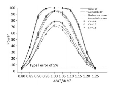
We also investigated the impact of variance and intra-correlation on the power of the Fieller-type confidence interval. Figure 1 presents the smoothed power curves with the CVs ranging from 0.8 to 1.6. The empirical power curves were drawn from log-normal-distribution data. The power of the Fieller-type confidence interval increased with the decrease of the CVs. The difference between empirical power and power function values became diminished significantly when the CVs of AUCs decreased from 1.2 to 0.6. The intra-correlation of AUCs had a positive correlation with the power of the bioequivalence test, as shown in Figure 2. The increase of intra-correlation did not cause an increase of difference between empirical power and power-function values. In all scenarios, the difference became minor when the values of the power function were larger than 80%.

Figure 1. Empirical power curves of Fieller-type confidence interval based on log-normal data and the function values of Fieller-type power and asymptotic power with different CVs. The intra-correlation was r = 0.6.
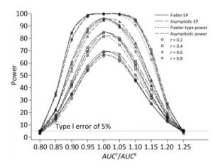
Figure 2. Empirical power curves of Fieller-type confidence interval based on log-normal data and the function values of Fieller-type power and asymptotic power with different intra-correlations. The coefficient of variance was CV = 1.2.
We observed that in all of the scenarios, Fieller-type power and asymptotic power were lower than the corresponding empirical power drawn from log-normal data. Thus, both the Fieller-type power function and asymptotic power function provided conservative estimations of the power of the bioequivalence test. When the ratios of two AUCs were larger than or equal to 1, asymptotic power was larger than the Fieller-type power. However, this trend was inversed when the ratio was less than 1.
-
In this work, we present a hypothetical example in order to demonstrate bioequivalence assessment and power analysis of the Fieller-type confidence interval, as well as sample size determination. In this example, we supposed that a two-sequence, two- period, two-treatment crossover study was conduc- ted to evaluate the bioequivalence of a follow-up azithromycin eye drop product to a reference product. The example data were constructed by selecting historical data from different trials conducted by the authors. All of these trials had ethical approvals. In these trials, a single dose of test or reference product (azithromycin eyedrop, 25 mg/2.5 mL) was instilled into each eye of each subject. An identical serial sampling regime was applied in these trials: tears were sampled at 0.17, 0.5, 2, 4, 8, 12, 24, and 36 hours after dosing. Sample methods, analytical methods, as well as demographics of subjects were also identical in these trials.
We consider this hypothetical example as a pilot study, in which six subjects were selected for each time point nested in each sequence. Table 3 presents the estimated AUCs for each sequence and period. The ratio AUCT/AUCR yielded 0.9142, the 90% Fieller-type confidence interval was (0.68851, 1.2628), and the 90% asymptotic confidence interval was (0.64602, 1.1823). The sample size was calculated using the R code given in Supplementary File S1. A total of 704 subjects (44 per timepoint in each sequence) were needed to achieve 80% power for a Fieller-type confidence interval.
Sequence Period 1 Period 2 Sequence (TR) 96022.94 104076.84 Sequence (RT) 147931.16 141684.28 Table 3. AUC Estimates for Each Sequence and Period
Simulation Study
Experimental Example
-
In the development of generic topical ophthalmic drugs, serial sampling is the most common sampling scheme due to the limitations of low bioavailability and difficulties in sampling. Although parametric methods for bioequivalence assessment in crossover designs with serial sampling data have been developed[14, 16], methods for sample-size determination are still limited. In this paper, we derived the power function of the Fieller-type confidence interval and the power function of the asymptotic confidence interval in crossover designs with serial sampling data. Simulation studies revealed that both the Fieller-type power function and the asymptotic power function could provide a reliable estimate for the power of bioequivalence assessment when normality assumptions were satisfied, as the values of both power functions were very close to the corresponding empirical power drawn from normal data. Moreover, both the Fieller-type power function and the asymptotic power function would yield a conservative estimate of power in cases when the study data were log-normally distributed. Both of the two power functions could be applied in power analysis for bioequivalence assessment.
Our derived power functions provide a simple way for determination of sample size in bioequivalence assessment using crossover design with serial sampling data. In current practice, bootstrap methods are most frequently used in bioequivalence assessment of generic topical ophthalmic drugs[4]. The sample size determination for bootstrap methods is a time-consuming process since it is carried out through batches of simulation studies. Through numerical iteration methods, the sample size for the Fieller-type confidence interval and the asymptotic confidence interval can be determined by the Fieller-type power function and the asymptotic power function, respectively. We recommend the use of the Fieller-type power if the expected ratio of AUCs is less than or equal to 1 since, in such case, the power of the Fieller-type confidence interval is larger than the asymptotic confidence interval. If the expected ratio of AUCs is larger than 1, the asymptotic confidence interval should be used since it has larger power. In practice, it might be difficult to make assumptions on the expected ratio of AUCs, especially without a previous pilot study. We consider that Fieller-type power could be preferable when the information on the test product is limited because the Fieller-type interval shows more robustness than the asymptotic interval in some extreme cases, such as when the variance of reference drug is too large, as suggested by Hirschberg et al.[26] Also, it would be reasonable to assume that the relative bioavailability, e.g., the ratio of AUCs, is less than 1 in study design. To avoid a waste of resources due to the overestimate of sample size, we suggest that the nominal power should be at least 80% since the difference between empirical power and power function value would be minor due to log normality.
In vivo bioequivalence studies for topical ophthalmic drugs are often conducted using a large sample size. Harigaya et al.[4] reviewed six bioequivalence studies of topical ophthalmic corticosteroid suspensions submitted to the FDA and showed that the numbers of subjects in each time point are around 70. Shen and Machado[15] illustrated a bioequivalence study of Tobradex AF suspension and TOBRADEX ophthalmic suspension, in which 987 subjects (at least 75 patients per timepoint) were enrolled to establish bioequivalence. This is because, in a serial sampling design, each subject must be involved in only one time point, and the AUC would be a linear combination of the average concentration of each time point. Correspondingly, the variance of the AUC would be a weighted sum of the variance of each time point, and the sample size needed to demonstrate bioequivalence would be consequently large. Thus, adaptive designs that allow early stopping or sample size reestimation would be preferable because of their advantage with respect to resource-saving or increasing the chances of eventual success. Based on our derived power functions, the conditional power function[29] and conditional target power[30], which are essential to adaptive adjustment, can be derived. With the power function of bioequivalence tests for the crossover trials with serial sampling design, adaptive designs-such as adaptive sample size sequential methods[31] and multiple-stage adaptive designs[32-34]-could be further considered in the context of serial sampling design.
-
The Fieller-type power function and the asymptotic power function can provide precise power estimates when normality assumptions are satisfied, and they may yield conservative estimates of power in cases when data are log-normally distributed. With these power functions, the sample size needed for bioequivalence assessment using crossover design with serial sampling data can be determined through numerical iteration methods. Adaptive sample size sequential methods and multiple-stage adaptive designs for crossover designs with serial sampling schemes could be cultivated further based on the derived power functions.
Supplementary File S1: Owen's Q function.
In this paper, we use Owen's Q function to calculate the cumulative density of a bivariate non-central t-distribution. The structure of Owen's Q function is shown below:
$$ \begin{array}{l} Q\left( {{t_1}, {t_2}, {\varphi _1}, {\varphi _2}, \rho } \right) = \frac{{\sqrt {2{\rm{ \mathsf{ π} }}} }}{{\mathit{\Gamma} \left( {\nu /2} \right){2^{\left( {\upsilon - 2} \right)/2}}}}\int_0^\infty {\mathit{\Phi} _2}(\frac{{{t_1}x}}{{\sqrt \upsilon }}\\ \;\;\;\;\;\;\;\;\;\;\;\;\;\;\;\;\;\;\;\;\;\;\;\;\;\;\; - {\varphi _1}, \frac{{{t_2}x}}{{\sqrt \upsilon }} - {\varphi _2}, \rho ){x^{\upsilon - 1}}\mathit{\Phi} '\left( x \right)dx, \end{array} $$ (25) $$\begin{array}{l} {\mathit{\Phi} _2}\left( {x, y, \rho } \right)\\ = \frac{1}{{2{\rm{ \mathsf{ π} }}\sqrt {\left( {1 - {\rho ^2}} \right)} }}\int_{ - \infty }^x \int_{ - \infty }^y {\rm{exp}}\left( { - \frac{{{u^2} - 2\rho u\upsilon + {\upsilon ^2}}}{{2\left( {1 - {\rho ^2}} \right)}}} \right)dudv, \\ \;\;\;\;\;\;\;\;\;\;\;\;\;\mathit{\Phi} '\left( x \right) = \frac{1}{{\sqrt {2\pi } }}{\rm{exp}}\left( { - \frac{{{x^2}}}{2}} \right) \end{array}$$ (26) where v is the degrees of freedom obtained using Satterthwaite approximation, φ1, φ2 are non-centrality parameters, and $\rho $ is correlation coefficient.
-
We thank LetPub (www.letpub.com) for its linguistic assistance during the preparation of this manuscript.
-
YY carried out the derivation, performed the data analysis and drafted the manuscript. JX conceived of research questions and revised the manuscript. YY, XY, and CY designed and performed the simulation study. XY and CY critically commented and revised the manuscript. All authors read and approved the final version of the manuscript.
-
power.serialsample<- function(auc=1, var.auc=1, cov.auc=1, nq=1)
{
t.auc<-auc[1];
r.auc<-auc[2];
t.aucse2<-var.auc[1]/nq;
r.aucse2<-var.auc[2]/nq;
cov.aucse<-cov.auc/nq;
feiller.t1<-(t.auc-0.80*r.auc)/sqrt(t.aucse2+0.80^2*r.aucse2-2*0.80*cov.aucse);
feiller.t2<-(t.auc-1.25*r.auc)/sqrt(t.aucse2+1.25^2*r.aucse2-2*1.25*cov.aucse);
corr.t1t2<-
(t.aucse2+0.80*1.25*r.aucse2-(0.80+1.25)*cov.aucse)/sqrt((t.aucse2+0.80^2*r.aucse2-2*0.80*cov.aucse)*(t.aucse2+1.25^2*r.aucse2-2*1.25*cov.aucse));
theta<-t.auc/r.auc;
df=(t.aucse2+theta^2*r.aucse2)^2/(t.aucse2^2/(2*nq-2)+theta^4*r.aucse2^2/(2*nq-2));
asy.se<-sqrt((t.aucse2+theta^2*r.aucse2-2*theta*cov.aucse)/r.auc^2);
asy.t1=(theta-0.80)/asy.se;
asy.t2=(theta-1.25)/asy.se;
powerasy.lower<-1-pt(qt(0.95, df), df, asy.t1);
powerasy.upper<-pt(-1*qt(0.95, df), df, asy.t2);
asy.power<-powerasy.upper+powerasy.lower-1;
library(mvtnorm)
delta<-c(feiller.t1, feiller.t2);
df<-as.integer(df);
rho<-corr.t1t2;
corr<-diag(2);
corr[1, 2]<-corr[2, 1]<-rho;
upper<-c(Inf, 0);
upper[2]<- -qt(1-0.05, df);
power<-pmvt(upper=upper, delta=delta, corr=corr, df=df);
upper[1]<- qt(1-0.05, df);
power<- power-pmvt(upper=upper, delta=delta, corr=corr, df=df);
fieller.power<-power;
result<-data.frame(feiller.t1, feiller.t2, corr.t1t2, theta, df, asy.t1, asy.t2, asy.se, fieller.power, asy.power);
return(result[c("fieller.power", "asy.power")])
}
-
npergroup.serialsample<- function(auc=1, var.auc=1, cov.auc=1, target.power=0.8, ci.method="fieller")
{
nq<-5;
if (!(tolower(ci.method) %in% c("fieller", "asymptotic"))){
warning("Method unkown. Will use the lower one the Fieller-type power and the Asymptotic power.\n", call.=FALSE, immediate.=TRUE)
}
method.list<-c("Fieller-type power", "Asymptotic power");
repeat{
if (tolower(ci.method)=="fieller"){
method.flag=1;
calc.power<-power.serialsample(auc=auc, var.auc=var.auc, cov.auc=cov.auc, nq=nq)[method.flag];
power.method<-method.list[1];
}
if (tolower(ci.method)=="asymptotic"){
method.flag=2;
calc.power<-power.serialsample(auc=auc, var.auc=var.auc, cov.auc=cov.auc, nq=nq)[method.flag];
power.method<-method.list[2];
}
if (!(tolower(ci.method) %in% c("fieller", "asymptotic"))){
calc.power<-power.serialsample(auc=auc, var.auc=var.auc, cov.auc=cov.auc, nq=nq);
method.flag=which.min(calc.power);
calc.power<-calc.power[which.min(calc.power)];
power.method<-method.list[method.flag];
}
nq<-nq+1;
if(calc.power[1]>=0.8){
npergroup<-nq-1;
target.power<-calc.power;
names(target.power)<-"Power";
break
}
}
result<-data.frame(power.method, target.power, npergroup);
return(result)
}
p1<-npergroup.serialsample(auc=c(118853.61, 126004.00), var.auc=c(1489997446.5, 3109615770.9), cov.auc=815789682.12, target.power=0.8, ci.method="fieller")
p2<-npergroup.serialsample(auc=c(118853.61, 126004.00), var.auc=c(1489997446.5, 3109615770.9), cov.auc=815789682.12, target.power=0.8, ci.method="asymptotic")
Program 1. R program for calculating the power of the Fieller-type confidence interval and the asymptotic confidence interval
Program 2. R program for calculating the sample size per timepoint for bioequivalence using the Fieller-type confidence interval or the asymptotic confidence interval
sub-project of National Major Scientific and Technological Special Project of China for 'Significant New Drugs Development' 2015ZX09501008-004

 Quick Links
 DownLoad:
