

 下载:
下载:


-
Metabolic syndrome (MS) is a common metabolic disorder status and defined as a pathology characterized by abdominal obesity, insulin resistance, hypertension, and hyperlipidemia (atherosclerosis) status[1]. Evidence suggests that the underlying etiology of MS is multifactorial and includes environmental factors, tobacco use, high alcohol consumption, dietary risks, and low physical activity. Thus, a deeper understanding of MS and its risk factors will be beneficial for mitigating health damage and improving the quality of life in high-risk subpopulations. PM2.5 is an important environmental pollutant, poses a serious threat to human health, and is associated with various health problems. Several epidemiological studies have shown that exposure to PM2.5 may influence the development of diabetes[2], cardiovascular disease, obesity, and MS. Existing evidence also suggests that the components of MS are sensitive to environmental pollutants, especially PM2.5. However, most of them were observational studies or literature analyses based on epidemiology, and the evidence for the causal association between PM2.5, MS, and its components remains limited. Mendelian randomization (MR), as a robust tool for making causal inferences, has been widely used in causal inference and can also overcome the limitations of observational studies. It uses single nucleotide polymorphisms (SNPs) that are closely related to exposure factors as instrumental variables to avoid the effects of confounding factors and reverse causation. As gametes follow the Mendelian laws of inheritance at formation, random assignment of alleles at conception eliminates confounding bias and follows the temporal nature of causation. Motivated by the above discussion, in this study, we first performed a two-sample MR analysis to determine the association between PM2.5, MS, and its components, using summary-level Genome-Wide Association Studies (GWAS) datasets. Multivariable MR analysis was carried out to adjust for the effect of several potential factors on the association between PM2.5 and MS. Furthermore, mediation MR analysis was used to verify the mediators that modified the association between PM2.5 and MS.
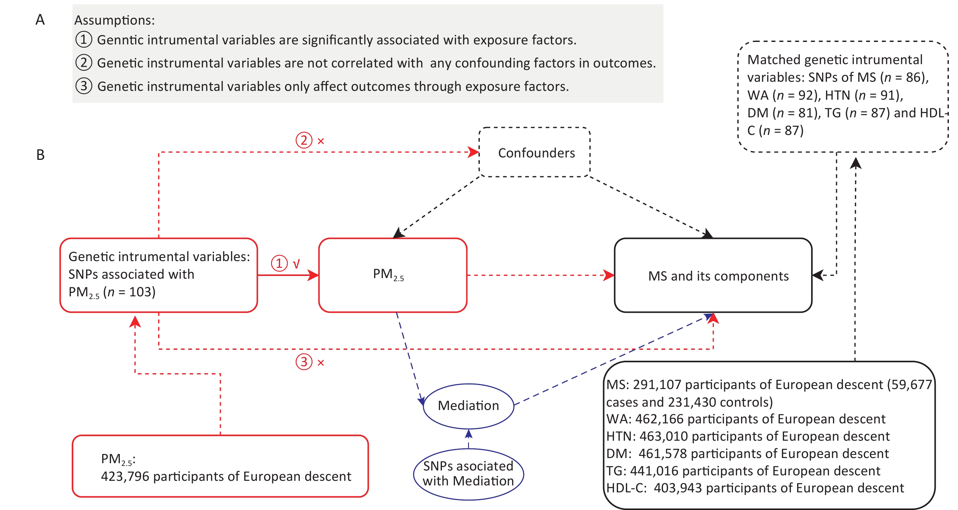
According to the International Diabetes Federation (IDF) criteria for the metabolic syndrome, MS consists of five components, namely waist circumference (WA, European, male: > 94 cm, female: > 80 cm), blood pressure/hypertension (HT, systolic pressure: > 130 mmHg or diastolic pressure: > 85 mmHg), diabetes mellitus (DM, FBG: > 5.6 mmol/L), triglycerides (TG, > 1.7 mmol/L) and high-density lipoprotein cholesterol (HDL-C, male: < 0.9 mmol/L, female: < 1.1 mmol/L). For the PM2.5, pooled genetic data were obtained from the UK Biobank GWAS (GWAS ID: ukb-b-10817), which included 423,796 European participants. This study was based on the European Cohort Study of Air Pollution Effects (ESCAPE project) and used land use regression (LUR model) to assess PM2.5 concentrations in participants’ residences. Summary-level data for MS were also available from the UK Biobank GWAS[3] (GWAS ID: ebi-a-GCST009602) and consisted of 291,107 individuals (59,677 cases and 231,430 controls). These data are the result of a GWAS analysis, aimed at exploring the relationship between population SNP and metabolic syndrome at the genetic level and constructing a correlation dataset between SNP and disease characterization, with genotypes, effect gene frequencies, effect coefficients for outcomes, and P values in the dataset. A summary of the genome-wide association data used in this study is presented in Supplementary Table S1 (available in www.besjournal.com).
Table S1. Summary description of genome-wide association data used in this study
Exposure/Outcome GWAS-ID Population N-cases (people) Sample size (people) Number of SNPs PM2.5 ukb-b-10817 European − 423,796 9,851,867 Mets ebi-a-GCST009602 European 59,677 291,107 9,463,307 WA ukb-b-9405 European − 462,166 9,851,867 HTN ukb-b-12493 European 54,358 463,010 9,851,867 DM ukb-b-10753 European 22,340 461,578 9,851,867 TG ieu-b-111 European − 441,016 12,321,875 HDL-C ieu-b-109 European − 403,943 12,321,875 The MR study was developed based on the instrumental variables (IVs). Single-nucleotide polymorphisms (SNPs) from the exposure dataset were used as genetic IVs. As listed in Figure 1, an MR study was conducted based on the three basic assumptions of IVs (more details can be found in Figure 1A). We chose P < 1 x 10⁻⁵ as the screening criterion for IVs. In addition, the function of the extraction instruments in the two-sample MR package was used to exclude contiguous imbalance (R2 < 0.001, window distance > 10,000 kb) when the exposed SNPs were included. In addition, we used the Pheno Scanner tool to identify and exclude SNP nucleotide polymorphisms significantly associated with PM2.5 which may affect MS through other biological pathways.
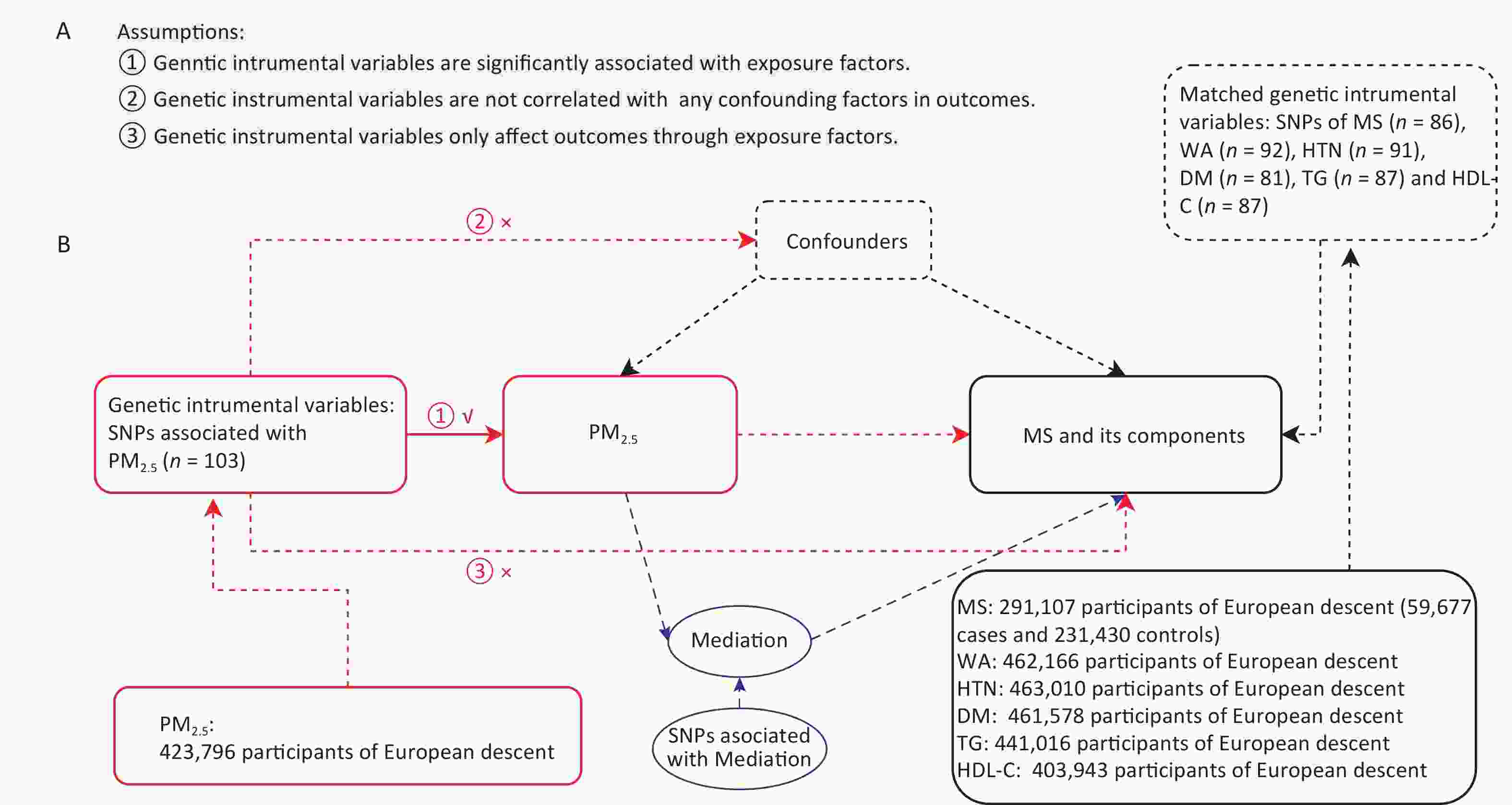
Figure 1. Mendelian randomization study design for PM2.5 and MS. (A) Mendelian randomization analysis based on three basic assumptions. (B) Flowchart of study design. MS, metabolic syndrome; WA, waist circumference; HT, hypertension; DM, diabetes mellitus; TG, triglyceride; HDL-C, high-density lipoprotein cholesterol.
A flowchart of the two-sample MR design is shown in Figure 1. The GWAS database summary-level data on PM2.5, MS, and its components were collected from the IEU-GWAS and GWAS catalogs, respectively, and two-sample MR analyses were performed to assess the association of PM2.5, MR, and its components based on the genetic IVs. Inverse variance weighting (IVW) is a standard method used in Mendelian randomization analysis. In the IVW method, the existence of intercept terms is not considered and the influence of each instrumental variable is assigned a weight that is the reciprocal of its variance. The MR-Egger was modified based on IVW, allowing for multi-validity detection while considering the presence of the intercept terms. The weighted median, simple mode, and weighted mode are commonly used estimation methods in Mendelian randomization. MR-Egger regression was used to analyze pleiotropy, testing for the presence of pleiotropic SNPs in the IVs (intercept close to 0 or P > 0.05, indicating no multiplicity[4]). The Cochran’s Q statistic for MR-Egger and IVW was used to test for heterogeneity between IVs.
In the multivariate MR analysis, we accounted for some potential life habits for consolidation and adjustment of the causal relationship between PM2.5 and MS, including smoking, alcohol intake frequency, and depressed mood[5-7], and used the IVW method for multivariate MR analysis. Multiple comparisons were corrected using the Bonferroni correction method, and the critical P-value was determined by the number of confounding exposures e as follows: P = 0.05/e. Furthermore, we also performed a mediation MR analysis (two-step MR) to validate and analyze the mediators that indirectly affected the association between PM2.5 and MS.
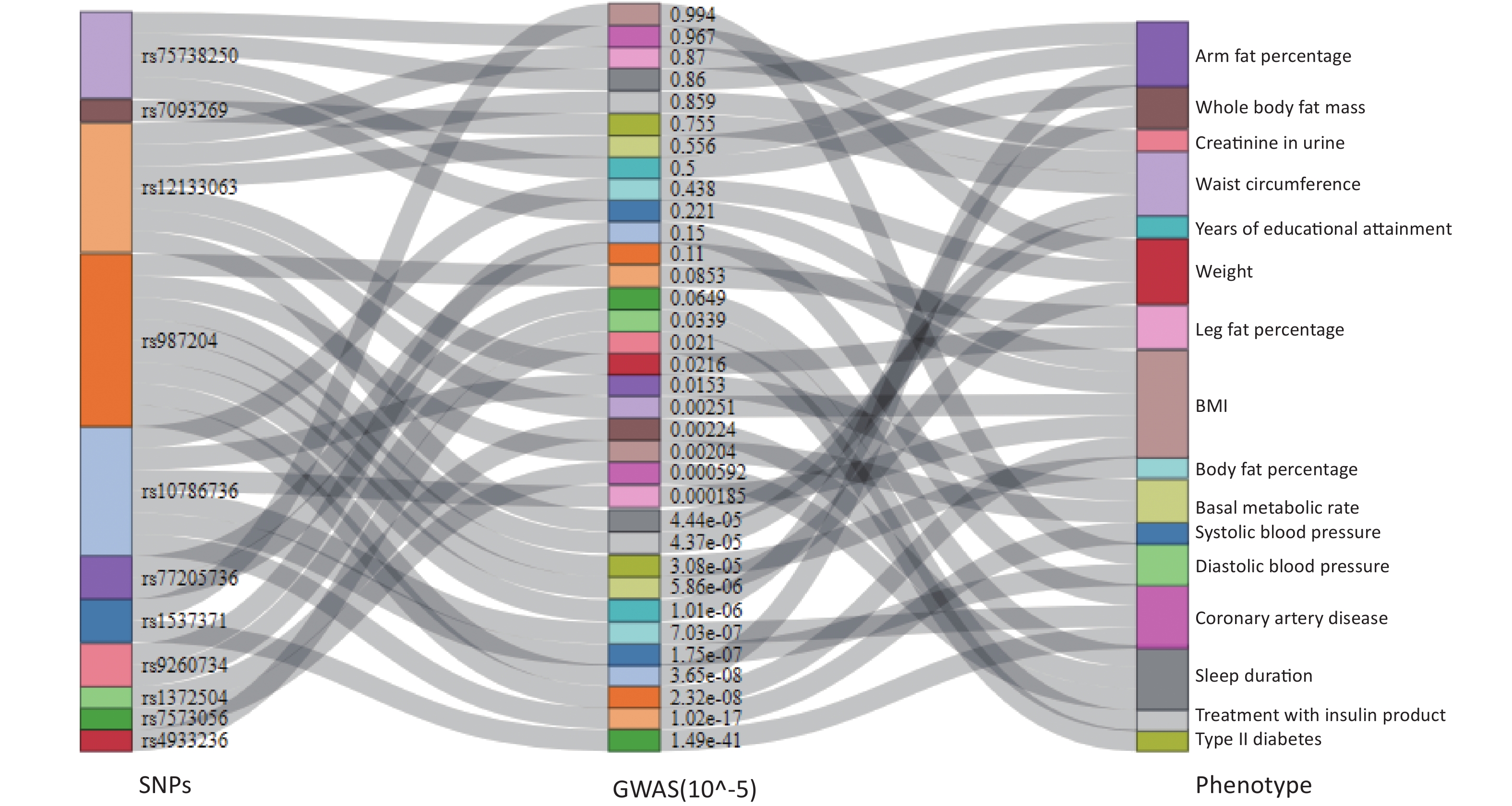
After excluding linkage disequilibrium (R2 = 0.001, kb = 10,000), we extracted 103 SNPs corresponding to PM2.5 from the GWAS dataset based on the criterion of P < 1 x 10⁻⁵. At the same time, 11 SNPs were associated with possible mechanistic pathways to MS (such as BMI, adiposity, and coronary heart disease); thus, these 11 SNPs were excluded from validation using the Pheno Scanner tool (Supplementary Figure S1 and Supplementary Table S2, available in www.besjournal.com) according to the basic assumptions of IVs (iii). Finally, 92 SNPs were identified for further MR analyses (Supplementary Table S3 and Supplementary Table S4, available in www.besjournal.com).
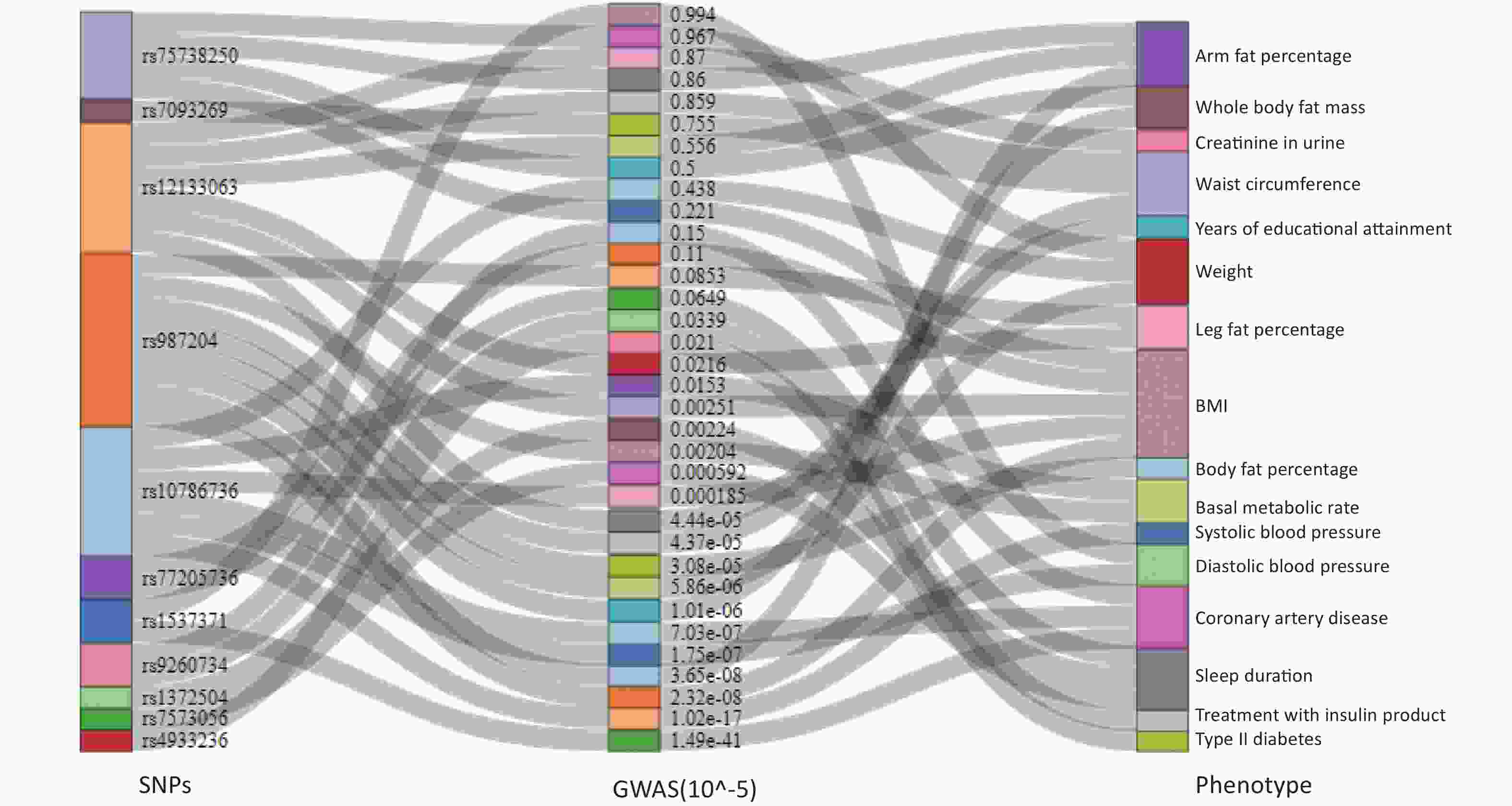
Figure S1. Sankey diagram for confounding factor analysis. 11 SNPs were excluded.
Table S2. Removed SNPs that may have other mechanistic pathways with MS
SNP EA OA PM2.5−BETA PM2.5−SE PM2.5−P value rs12133063 A C 0.01044 0.002265 4.00 x 10⁻⁶ rs7573056 C A −0.01141 0.00217 1.50 x 10⁻⁷ rs987204 A G 0.010299 0.002167 2.00 x 10⁻⁶ rs75738250 A T 0.013337 0.00294 5.70 x 10⁻⁶ rs1372504 A G 0.012291 0.002219 3.10 x 10⁻⁸ rs9260734 A G 0.013983 0.003 3.10 x 10⁻⁶ rs77205736 T C 0.013522 0.002413 2.10 x 10⁻⁸ rs1537371 A C 0.012371 0.002149 8.50 x 10⁻⁹ rs4933236 C T 0.01001 0.002202 5.50 x 10⁻⁶ rs10786736 C G 0.015813 0.003571 9.50 x 10⁻⁶ rs7093269 A T 0.179809 0.04032 8.20 x 10⁻⁶ Table S3. Mendelian randomisation information for PM2.5 and MS
Exposure Outcome No. snp R2 F-statistics PM2.5 MS 86 0.458% 22.585 PM2.5 WA 92 0.490% 22.591 PM2.5 HT 91 0.482% 22.453 PM2.5 DM 81 0.431% 22.589 PM2.5 TG 87 0.460% 22.418 PM2.5 HDL-C 87 0.460% 22.418 Table S4. GWAS reported PM2.5 with MS summary statistics after MR analysis using SNPs
SNP EA OA PM2.5 MS F BETA SE P BETA SE P rs10203969 T G −0.01031 0.00227 5.50 x 10⁻⁶ −0.0058 0.006897 0.40026 20.63 rs10961167 A G −0.01934 0.004066 2.00 x 10⁻⁶ −0.01468 0.012346 0.234455 22.62 rs11042316 A G −0.01304 0.002498 1.80 x 10⁻⁷ 0.010394 0.007567 0.169538 27.25 rs11075636 G A −0.0131 0.002948 8.90 x 10⁻⁶ −0.00935 0.008955 0.296563 19.75 rs11209977 G A 0.013974 0.003145 8.90 x 10⁻⁶ 0.015261 0.009464 0.106844 19.74 rs114708313 T A 0.024558 0.004478 4.20 x 10⁻⁶ 0.013396 0.014024 0.339479 30.08 rs11610713 T A 0.03797 0.008066 2.50 x 10⁻⁶ 0.043792 0.024146 0.069735 22.16 rs11616726 G T −0.01765 0.003976 9.00 x 10⁻⁶ 0.002241 0.011965 0.851418 19.71 rs116259394 G A −0.03491 0.007841 8.50 x 10⁻⁶ −0.00688 0.023712 0.771641 19.82 rs116925111 G T 0.053321 0.010861 9.10 x 10⁻⁷ −0.01222 0.032699 0.70865 24.10 rs1172955 A T 0.010736 0.002368 5.80 x 10⁻⁶ 0.00328 0.007207 0.649014 20.56 rs117366154 T C −0.01933 0.00428 6.30 x 10⁻⁶ −0.0184 0.013078 0.159458 20.40 rs117878224 G A −0.04804 0.010066 1.80 x 10⁻⁶ −0.00571 0.031121 0.854417 22.78 rs1182891 T G 0.012738 0.002773 4.40 x 10⁻⁶ 0.002311 0.008448 0.784398 21.10 rs11855821 A G −0.01262 0.002432 2.10 x 10⁻⁷ −0.03074 0.007401 3.27 x 10⁻⁵ 26.93 rs1217106 G A 0.012725 0.00262 1.20 x 10⁻⁶ −0.01932 0.00792 0.014705 23.59 rs12203592 T C 0.021666 0.002591 6.20 x 10⁻¹⁷ −0.00314 0.008113 0.698962 69.92 rs12812511 G A 0.011141 0.002391 3.20 x 10⁻⁶ −0.00292 0.007275 0.688603 21.71 rs13035717 T A −0.01306 0.00285 4.60 x 10⁻⁶ 0.006577 0.008602 0.444484 21.00 rs1318845 C T −0.01397 0.002699 2.30 x 10⁻⁷ −0.00563 0.008211 0.492554 26.79 rs1340247 A G −0.00994 0.002212 7.00 x 10⁻⁶ 0.000387 0.006712 0.95405 20.19 rs13429081 T A 0.013647 0.002777 8.90 x 10⁻⁷ 0.013627 0.008416 0.10542 24.15 rs138685951 T C −0.03082 0.006786 5.60 x 10⁻⁶ 0.017101 0.020402 0.401925 20.63 rs140500108 G C −0.02217 0.004871 5.30 x 10⁻⁶ −0.01518 0.014663 0.300606 20.72 rs147392452 T C −0.0282 0.006333 8.50 x 10⁻⁶ 0.027389 0.018821 0.145602 19.83 rs151323121 A G −0.0416 0.0092 6.10 x 10⁻⁶ −0.00978 0.02845 0.731069 20.45 rs16957755 C T 0.021686 0.004384 7.60 x 10⁻⁷ 0.015536 0.013297 0.242639 24.47 rs17070492 G C 0.016888 0.003617 3.00 x 10⁻⁶ 0.010552 0.010986 0.336791 21.80 rs17103928 A C −0.01393 0.003009 3.70 x 10⁻⁶ 0.010238 0.009144 0.262898 21.43 rs17183854 G T −0.04343 0.00942 4.00 x 10⁻⁶ −0.00357 0.02897 0.901804 21.26 rs17657881 C T −0.03711 0.008046 4.00 x 10⁻⁶ 0.061092 0.023926 0.01067 21.27 rs1933805 A G 0.009601 0.002167 9.40 x 10⁻⁶ −0.00478 0.00658 0.467634 19.63 rs2091322 C T −0.00978 0.002201 8.80 x 10⁻⁶ −0.00767 0.00669 0.251746 19.74 rs2141531 G T −0.01142 0.002356 1.30 x 10⁻⁶ −0.00268 0.007168 0.708458 23.50 rs2278801 G A 0.010241 0.002268 6.30 x 10⁻⁶ −0.00549 0.006893 0.425917 20.39 rs2292156 T G 0.014681 0.002878 3.40 x 10⁻⁷ −0.00683 0.008738 0.434595 26.02 rs2324898 T C 0.010107 0.002256 7.50 x 10⁻⁶ 0.002215 0.00718 0.757716 20.07 rs27152 T C −0.01073 0.002305 3.20 x 10⁻⁶ −0.00437 0.006997 0.532724 21.67 rs35703574 A G −0.02468 0.005345 3.90 x 10⁻⁶ −0.01423 0.016071 0.375896 21.32 rs45485691 A G −0.01084 0.002414 7.20 x 10⁻⁶ −0.00342 0.007339 0.641473 20.16 rs4854523 G A 0.013445 0.002893 3.40 x 10⁻⁶ 0.003351 0.008788 0.702982 21.60 rs487230 G A −0.01164 0.002512 3.60 x 10⁻⁶ −0.01132 0.00761 0.137044 21.47 rs4926311 T C −0.01037 0.002325 8.20 x 10⁻⁶ −0.00512 0.007054 0.468343 19.89 rs56068671 T G −0.01819 0.003926 3.60 x 10⁻⁶ −0.02945 0.011997 0.014095 21.47 rs56181709 T C −0.01165 0.002593 7.10 x 10⁻⁶ −0.00701 0.007902 0.375032 20.19 rs58824859 C A 0.012008 0.002305 1.90 x 10⁻⁷ 0.00714 0.006996 0.307473 27.14 rs6024877 C T 0.024387 0.005511 9.70 x 10⁻⁶ −0.03231 0.017077 0.058485 19.58 rs62119705 T C 0.011135 0.002265 8.90 x 10⁻⁷ −0.00317 0.006867 0.644091 24.17 rs62180462 A G −0.03511 0.007628 4.20 x 10⁻⁶ 0.008711 0.022738 0.701656 21.19 rs62368672 C T −0.01812 0.003929 4.00 x 10⁻⁶ −0.00353 0.011893 0.766586 21.27 rs62484669 A G 0.017816 0.003621 8.60 x 10⁻⁷ 0.013731 0.010965 0.210459 24.21 rs628913 T C −0.00993 0.002182 5.40 x 10⁻⁶ 0.001452 0.006629 0.826637 20.71 rs6432776 C T 0.011436 0.002386 1.60 x 10⁻⁶ 0.016863 0.007288 0.020682 22.97 rs6547952 G T −0.01109 0.002283 1.20 x 10⁻⁶ 0.000258 0.006939 0.97036 23.60 rs656813 C T −0.01403 0.003158 8.90 x 10⁻⁶ 0.005149 0.009535 0.589181 19.74 rs66501886 G C −0.01025 0.002315 9.50 x 10⁻⁶ −0.00595 0.007026 0.397199 19.60 rs6667345 T C 0.011551 0.002562 6.50 x 10⁻⁶ −0.00167 0.007782 0.829871 20.33 rs6749467 A G −0.01239 0.002183 1.40 x 10⁻⁸ −0.00458 0.006634 0.49004 32.21 rs6937315 C T 0.010179 0.002252 6.20 x 10⁻⁶ 0.003826 0.006842 0.576051 20.43 rs6960011 G A −0.01052 0.002275 3.70 x 10⁻⁶ −0.00729 0.006899 0.290951 21.38 rs718059 A G −0.01351 0.002943 4.40 x 10⁻⁶ 0.006105 0.008937 0.49457 21.07 rs72655898 G A −0.01132 0.002398 2.40 x 10⁻⁶ −0.00162 0.007269 0.824006 22.28 rs72700006 C T 0.02003 0.004246 2.40 x 10⁻⁶ −0.01282 0.012926 0.321366 22.25 rs72805044 C T −0.03735 0.008346 7.60 x 10⁻⁶ −0.04117 0.025718 0.10946 20.03 rs72808024 C A −0.01609 0.00302 9.90 x 10⁻⁸ −0.00987 0.009142 0.280233 28.39 rs7514956 C A −0.01298 0.00276 2.60 x 10⁻⁶ 0.005202 0.008358 0.533667 22.12 rs75730485 C T −0.02677 0.006053 9.80 x 10⁻⁶ −0.0165 0.018266 0.366253 19.56 rs76230173 A G −0.02084 0.004655 7.60 x 10⁻⁶ −0.01283 0.014067 0.361743 20.04 rs77147615 C T 0.024822 0.005567 8.20 x 10⁻⁶ −0.00499 0.016932 0.768271 19.88 rs77255816 T C 0.031394 0.005728 4.20 x 10⁻⁸ 0.008359 0.017401 0.630984 30.04 rs7750418 G T 0.010366 0.002304 6.80 x 10⁻⁶ −0.00138 0.006995 0.843882 20.24 rs7776279 A G 0.010947 0.002385 4.40 x 10⁻⁶ −0.01132 0.007227 0.11737 21.07 rs77962859 C T −0.01575 0.003514 7.30 x 10⁻⁶ 0.004525 0.010717 0.672879 20.09 rs78230389 G A −0.04679 0.009485 8.10 x 10⁻⁷ −0.0282 0.028893 0.329133 24.33 rs78467598 G C −0.038 0.007686 7.60 x 10⁻⁷ −0.02073 0.023206 0.371763 24.44 rs78539764 C T −0.03352 0.00659 3.70 x 10⁻⁷ −0.01471 0.019967 0.46133 25.87 rs78546077 C T −0.03172 0.006923 4.60 x 10⁻⁶ −0.02824 0.020767 0.173861 20.99 rs79004040 G C −0.03223 0.007254 8.90 x 10⁻⁶ 0.021232 0.02176 0.329203 19.74 rs7910200 T C −0.00982 0.002175 6.30 x 10⁻⁶ 0.001309 0.006606 0.842972 20.38 rs79229868 A G 0.044548 0.009946 7.50 x 10⁻⁶ 0.026595 0.030306 0.380191 20.06 rs800507 T G 0.011213 0.002536 9.80 x 10⁻⁶ 0.021921 0.007697 0.004401 19.55 rs80123875 T G −0.01874 0.003867 1.30 x 10⁻⁶ −0.00078 0.011685 0.947048 23.48 rs80347400 G A 0.013727 0.003034 6.10 x 10⁻⁶ 0.020388 0.009151 0.025882 20.47 rs8614 A C 0.01308 0.00279 2.80 x 10⁻⁶ 0.005701 0.008463 0.500554 21.98 rs875982 T C −0.01005 0.002215 5.70 x 10⁻⁶ 0.001891 0.00672 0.778447 20.59 rs9644485 C T 0.009868 0.002159 4.90 x 10⁻⁶ −0.00751 0.006549 0.251328 20.89 The MR-Egger intercept analysis showed that there was no pleiotropy in the MR analysis of MS and its components (Supplementary Table S5, available in www.besjournal.com). The Cochran’s Q statistic for MR-Egger and IVW in the heterogeneity test suggested possible heterogeneity due to individual variations (PQ1 = 0.047, PQ2 = 0.054).
Table S5. Results of the test for multiplicity and heterogeneity of SNPs for PM2.5 in MS data
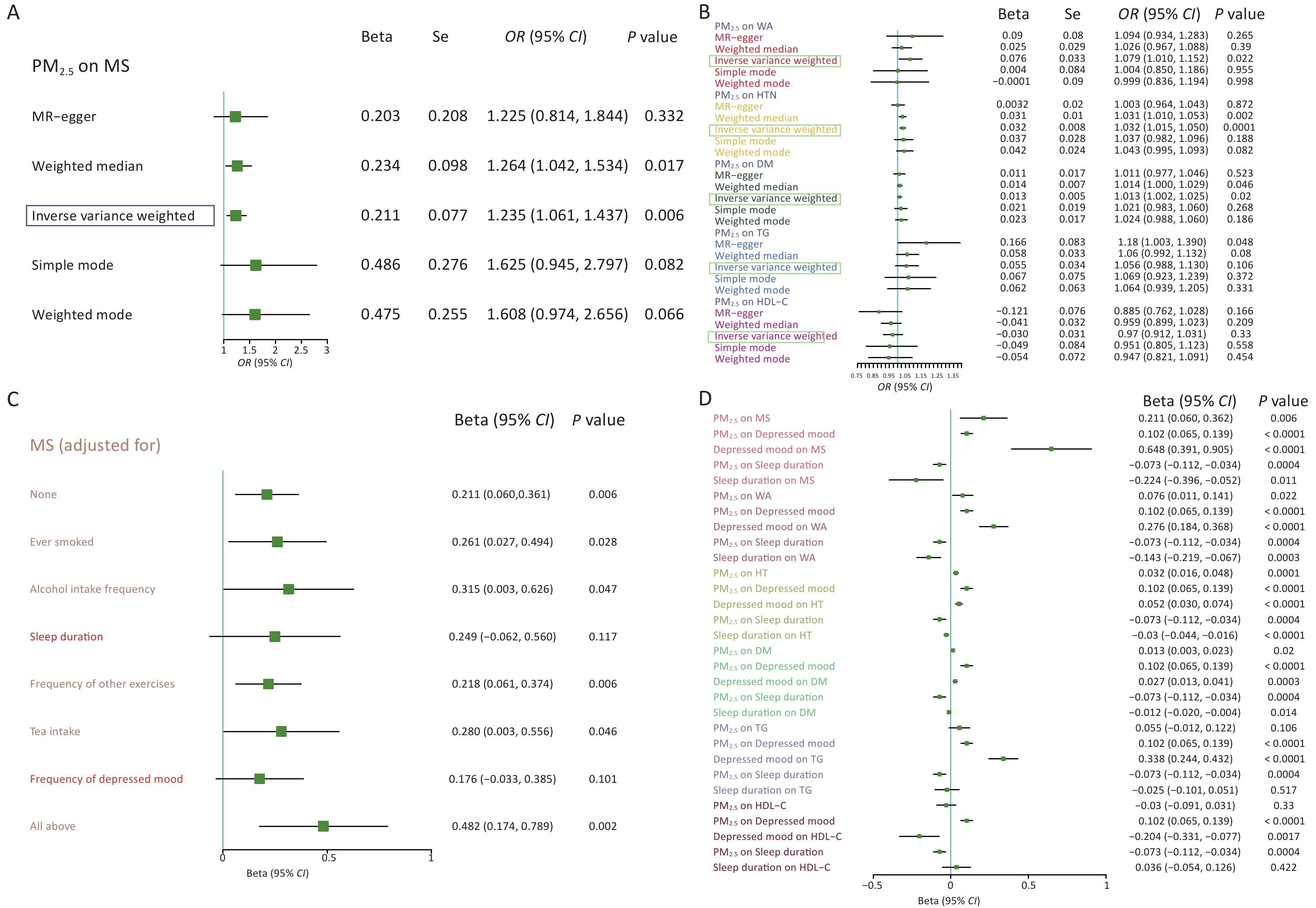
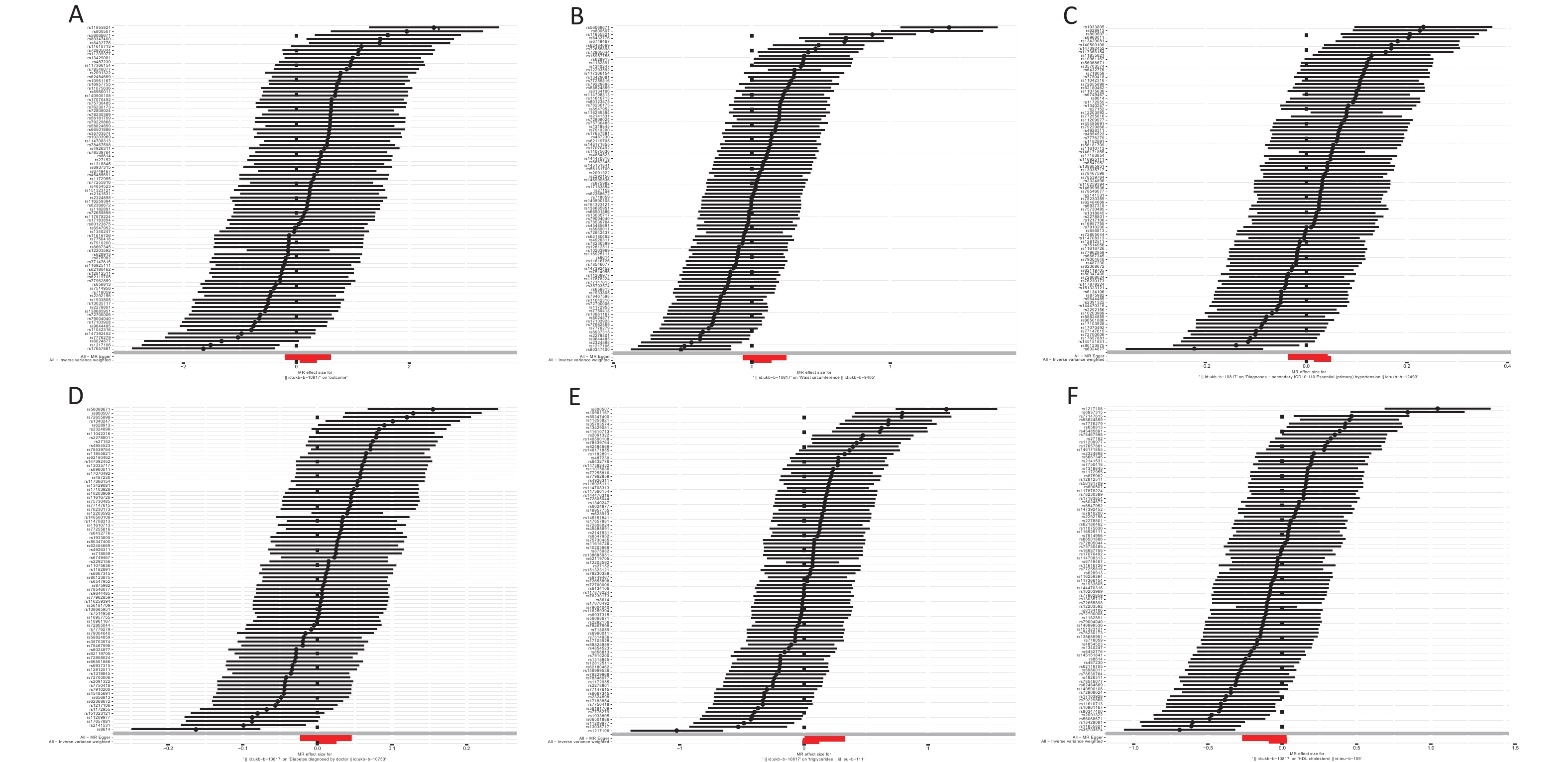
Index Pleiotropy test Heterogeneity test MR−egger MR−egger Inverse variance weighted Intercept SE P Q Q_df P Q Q_df P MS 0.00012 0.0029 0.966 106.833 84 0.0470 106.835 85 0.054 WA −0.00023 0.0011 0.842 305.630 90 2.869 × 10⁻²⁵ 305.765 91 5.077 × 10⁻²⁵ HT 0.00047 0.0002 0.113 143.187 89 0.0002 147.287 90 0.0001 DM 3.72 × 10⁻⁵ 0.0002 0.879 121.651 79 0.0014 121.686 80 0.0018 TG −0.00178 0.0012 0.147 225.044 85 1.319 × 10⁻¹⁴ 230.704 86 3.580 × 10⁻¹⁵ HDL−C 0.00146 0.0011 0.196 205.380 85 5.836 × 10⁻¹² 209.478 86 2.675 × 10⁻¹² The results of the two-sample MR analysis of the associations between PM2.5, MS, and their components are shown in Figure 2A–B, respectively. In the random-effects IVW model, MS may increase by 23.5% when the concentration of PM2.5 increases by one standard deviation (OR = 1.235, 95% CI: 1.061–1.437, P = 0.006). The MR-Egger, Simple mode, and weighted mode models also validated the direction of the causal association, which is consistent with the IVW model. Previous studies have shown that atmospheric pollutants such as PM2.5 have an impact on chronic diseases such as metabolic syndrome, and our results have confirmed this, further demonstrating the potential threat of PM2.5 to public health. For the MS components, these SNPs (genetic predictors of PM2.5) were positively correlated with WA, HT, and DM (all P < 0.05). More precisely, the random-effects IVW models indicated that the associated effects of PM2.5 on WA were OR = 1.079 (95% CI: 1.010–1.152, P = 0.022), 1.032 (95% CI: 1.015–1.050, P = 0.0001), and 1.013 (95% CI, 1.002–1.025; P = 0.020), respectively. This indicates that PM2.5, mainly reflected in obesity, blood sugar, and blood pressure, may affect multiple aspects of metabolic processes. There was no statistical correlation between the impact of PM2.5 on blood lipids, which may be due to the smaller impact of PM2.5 on these specific indicators or the need for larger sample sizes and more accurate methods for validation (Supplementary Table S6, available in www.besjournal.com). Supplementary Figure S2 (available in www.besjournal.com) shows the influence of individual SNPs on outcomes and their combined effect. As shown in Supplementary Figure S3 (available in www.besjournal.com), the leave-one-out tests also validated that the association between PM2.5, MS, and its components (WA, HT, and DM) was effective and robust. The funnel plot of Supplementary Figure S4 (available in www.besjournal.com) shows that the scatter is symmetrical, and the SNPs scatter plot of exposure and outcome is shown in Supplementary Figure S5 (available in www.besjournal.com).
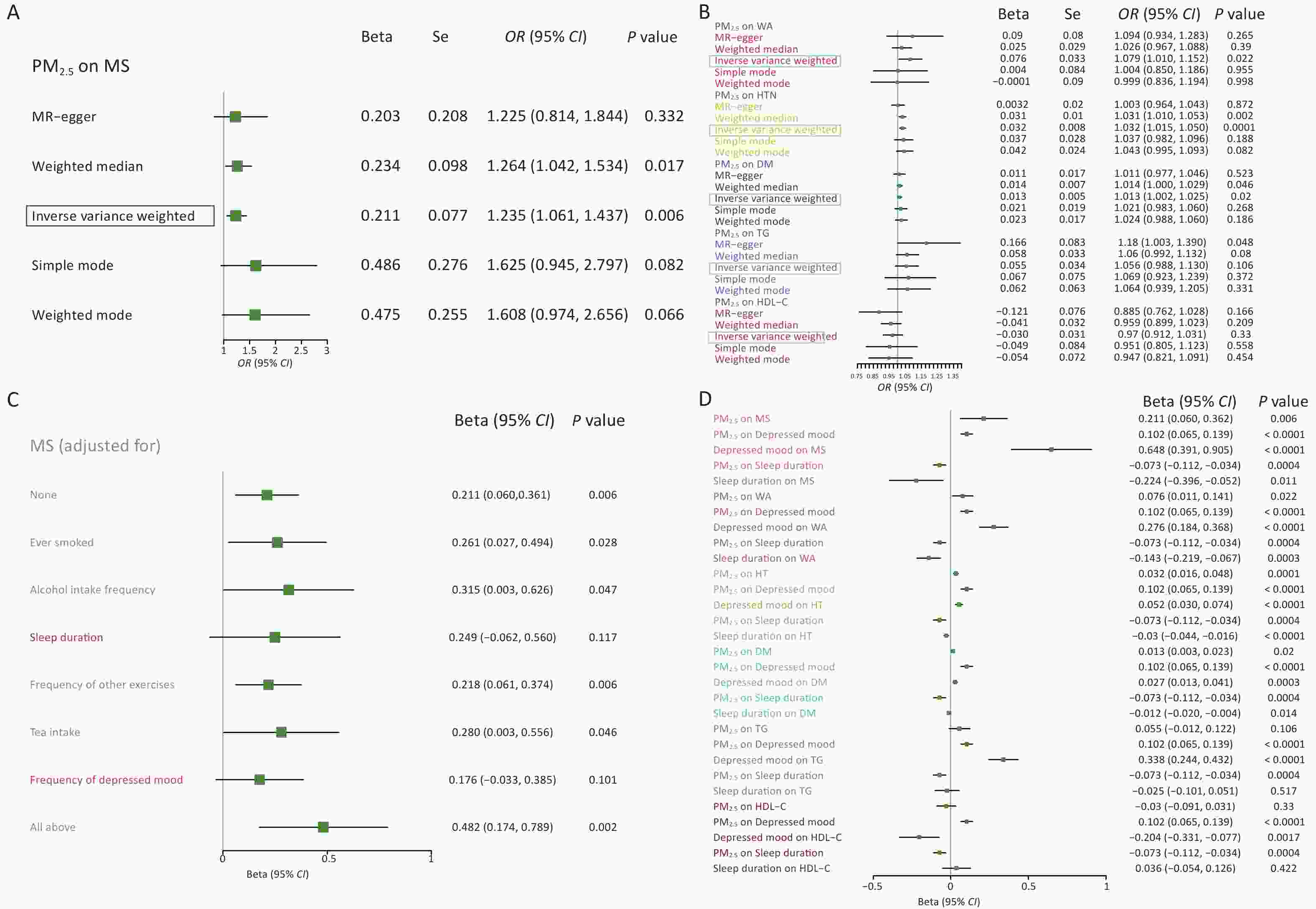
Figure 2. MR analysis results of PM2.5 on metabolic syndrome and components. (A) MR analysis results of the effects of PM2.5 on metabolic syndrome. (B) MR analysis results of PM2.5 on the components of MS. (C) Multivariate analysis of the impact of PM2.5 on metabolic syndrome. (D) Intermediary analysis of PM2.5 on metabolic syndrome and its components. MS, metabolic syndrome; WA, waist circumference; HT, hypertension; DM, diabetes mellitus; TG, triglyceride; HDL-C, high-density lipoprotein cholesterol; MR, Mendelian randomization.
We performed multivariate MR analysis to further evaluate the relationship between PM2.5 and MS after adjusting for several potential confounding factors (Figure 2C). After adjusting for these confounding factors such as ever smoked, alcohol intake frequency, sleep duration, frequency of exercise, tea intake, and depressed mood, the relationship between PM2.5 and MS still has significance (β = 0.482, P = 0.002). However, after adjusting for sleep duration and frequency of depressed mood, the relationship between PM2.5 and MS was not significant.
To further estimate the association between PM2.5 and MS based on the results of multivariate MR analysis, we also performed the Mediation analysis to assess the mediating effect of the sleep duration and frequency of depressed mood on the relationship between PM2.5 and MS. As given in Figure 2D, the result suggested that the causal effect of PM2.5 on MS may be partially mediated by frequency of depressed mood (approximately mediated by 31.32%, 95% CI: 13.06%–106.22%) and sleep duration (approximately mediated by 7.74%, 95% CI: 1.27%–31.60%), respectively. Furthermore, for the components of MS, the frequency of depressed mood mediated approximately 37.04% (95% CI: 14.52%–167.42%), 16.57% (95% CI: 7.30%–36.91%) and 21.18% (95% CI: 6.98%–80.25%) of the relationship between PM2.5 and WA, HT and DM, and the sleep duration mediated approximately 13.73% (95% CI: 3.69%–64.07%), 6.84% (95% CI: 2.51%–16.68%) and 6.73% (95% CI: 1.42%–28.49%) of the relationship between PM2.5 and WA, HT and DM. Interestingly, the relationship between PM2.5, TG, and HDL-C was completely mediated by the frequency of depressed mood, which may be one reason for the insignificant relationship between PM2.5, TG, and HDL-C levels.
As both PM2.5 and MS are risk factors for cardiovascular diseases, their relationship has attracted extensive attention in recent years. Previous epidemiological studies have shown that PM2.5 may be significantly and positively associated with the risk of developing metabolic syndrome. However, evidence for a causal association between PM2.5, MS, and its components remains limited. In this study, we first used a two-sample MR to analyze the causal association between PM2.5, MS, and its five components. Two-sample MR analysis results indicated that MS may increase by 23.5% excess risk when the concentration of PM2.5 increases by one standard deviation (OR = 1.235, 95% CI: 1.061–1.437), these results were consistent with some existing studies across different subpopulation and regions.
As for the five components of MS, Chen et al.[8] indicated that every 10-μg/m3 increase in annual PM2.5 concentration was associated with an increased risk of abdominal obesity, hypertriglyceridemia, low HDL-C, hypertension, and elevated fasting blood glucose by using a longitudinal cohort in Taiwan, China. Rachel et al.[9] used a Cox Proportional Risk model and found that each 1 μg/m3 increase in annual mean PM2.5 concentration was associated with an HR of 1.27 (95% CI: 1.06–1.52) for the risk of MS, and also influenced elevated fasting glucose and hypertriglyceridemia. Moreover, some studies have suggested that an increase in PM2.5 may be associated with increased waist circumference, HT, and the onset of diabetes. Consistent with this evidence, our two-sample MR analysis proposed that the associated effects of PM2.5 on WA were OR = 1.079 (95% CI: 1.010–1.152), 1.032 (95% CI: 1.015–1.050), and 1.013 (95% CI: 1.002–1.025), respectively.
Furthermore, mediation analysis of MR suggested that depression and sleep duration may play a mediating role in the association between PM2.5 and MS. The causal effect of PM2.5 on MS may be partially mediated by the frequency of depressed mood (approximately mediated by 31.32%) and sleep duration (approximately mediated by 7.74%). PM2.5 exposure may affect inflammation via the NLRP3 single pathway, which plays an important role in inducing depression. Sympathetic nervous system nerve excitation and release of pro-inflammatory factors caused by insufficient sleep lead to insulin resistance. By extension, public health strategies such as developing more rational emotional regulation and increasing sleep duration may be beneficial for mitigating the adverse effects of PM2.5.
The biological mechanisms linking PM2.5, MS, and its components are still limited, and some reasons may explain the relationship between PM2.5, MS, and its five components. First, the effect of PM2.5 on obesity may occur through systemic inflammation, altered energy metabolism, and other pathways. Secondly, abnormal energy metabolism is one of the causes[10]. Organisms exposed to PM2.5 may affect their own and their offspring’s energy balance by inducing brown adipose tissue (BAT) bleaching and regulating food intake, causing fat accumulation. Thirdly, many studies have shown that PM2.5 can affect blood sugar and blood pressure, including but not limited to inducing insulin resistance, promoting catecholamine release, and the Notch signaling pathway.
Our study has the following limitations. First, the GWAS data used for the study were from Europe; further studies on other national populations are needed to improve the generalizability of the results. The fact that the data for different components were obtained from different studies may also have led to bias in the results. Second, due to a lack of sufficient SNPs after linkage disequilibrium, we relaxed the P-value threshold (P < 1 x 10⁻⁵) of SNPs of PM2.5 in accordance with previous studies, which might have led to weak instrumental variables. To address this issue, we calculated the F-statistics to measure the power of each SNP. All SNPs used in the study with an F-statistic greater than 10 indicated the absence of weak instrument bias. Third, although the hypothesis of exclusivity was passed by the multiplicity test with the Phenoscanner search, we were unable to eliminate the potential multiplicity problem that may have arisen from the low number of instrumental variables. Based on the results of multivariate MR, possible mediating factors were selected; therefore, we did not conduct a separate multivariate MR analysis of the components of MS.
Our findings suggest that there may be a relationship between PM2.5 and MS. For the MS component, PM2.5 was more likely to affect the metabolic syndrome through waist circumference, hypertension, and hyperglycemia. Mediation MR analysis found that the association of PM2.5 with MS may be partially mediated by the frequency of depressed mood (approximately 31.32%) and sleep duration (approximately 7.74%). Our findings recommended that the prevention and management of PM2.5 might be enhanced for MS and its components prevention. Although these findings provide strong evidence, they should be interpreted cautiously. First, these studies were based on the genetic prediction of PM2.5, rather than directly measuring exposure levels. Therefore, these results may be influenced by the accuracy of genetic predictions. Second, these studies were based on specific population samples and may not fully represent the entire population. Therefore, these results must be validated in larger populations.
-
Not applicable.
-
Table S6. Two-sample Mendelian randomization results for PM2.5 and MS
Exposure Outcome Method Beta SE OR OR 95% CI P PM2.5 MS MR−egger 0.203 0.208 1.225 (0.814, 1.844) 0.332 Weighted median 0.234 0.098 1.264 (1.042, 1.534) 0.017 Inverse variance weighted 0.211 0.077 1.235 (1.061, 1.437) 0.006 Simple mode 0.486 0.276 1.625 (0.945, 2.797) 0.082 Weighted mode 0.475 0.255 1.608 (0.974, 2.656) 0.066 PM2.5 WA MR−egger 0.090 0.080 1.094 (0.934, 1.283) 0.265 Weighted median 0.025 0.029 1.026 (0.967, 1.088) 0.390 Inverse variance weighted 0.076 0.033 1.079 (1.010, 1.152) 0.022 Simple mode 0.004 0.084 1.004 (0.850, 1.186) 0.955 Weighted mode −0.0001 0.090 0.999 (0.836, 1.194) 0.998 PM2.5 HT MR−egger 0.0032 0.020 1.003 (0.964, 1.043) 0.872 Weighted median 0.031 0.010 1.031 (1.010, 1.053) 0.002 Inverse variance weighted 0.032 0.008 1.032 (1.015, 1.050) 0.0001 Simple mode 0.037 0.028 1.037 (0.982, 1.096) 0.188 Weighted mode 0.042 0.024 1.043 (0.995, 1.093) 0.082 PM2.5 DM/FBG MR−egger 0.011 0.017 1.011 (0.977, 1.046) 0.523 Weighted median 0.014 0.007 1.014 (1.000, 1.029) 0.046 Inverse variance weighted 0.013 0.005 1.013 (1.002, 1.025) 0.020 Simple mode 0.021 0.019 1.021 (0.983, 1.060) 0.268 Weighted mode 0.023 0.017 1.024 (0.988, 1.060) 0.186 PM2.5 TG MR−egger 0.166 0.083 1.180 (1.003, 1.390) 0.048 Weighted median 0.058 0.033 1.060 (0.992, 1.132) 0.080 Inverse variance weighted 0.055 0.034 1.056 (0.988, 1.130) 0.106 Simple mode 0.067 0.075 1.069 (0.923, 1.239) 0.372 Weighted mode 0.062 0.063 1.064 (0.939, 1.205) 0.331 PM2.5 HDL−C MR−egger −0.121 0.076 0.885 (0.762, 1.028) 0.166 Weighted median −0.041 0.032 0.959 (0.899, 1.023) 0.209 Inverse variance weighted −0.030 0.031 0.970 (0.912, 1.031) 0.330 Simple mode −0.049 0.084 0.951 (0.805, 1.123) 0.558 Weighted mode −0.054 0.072 0.947 (0.821, 1.091) 0.454 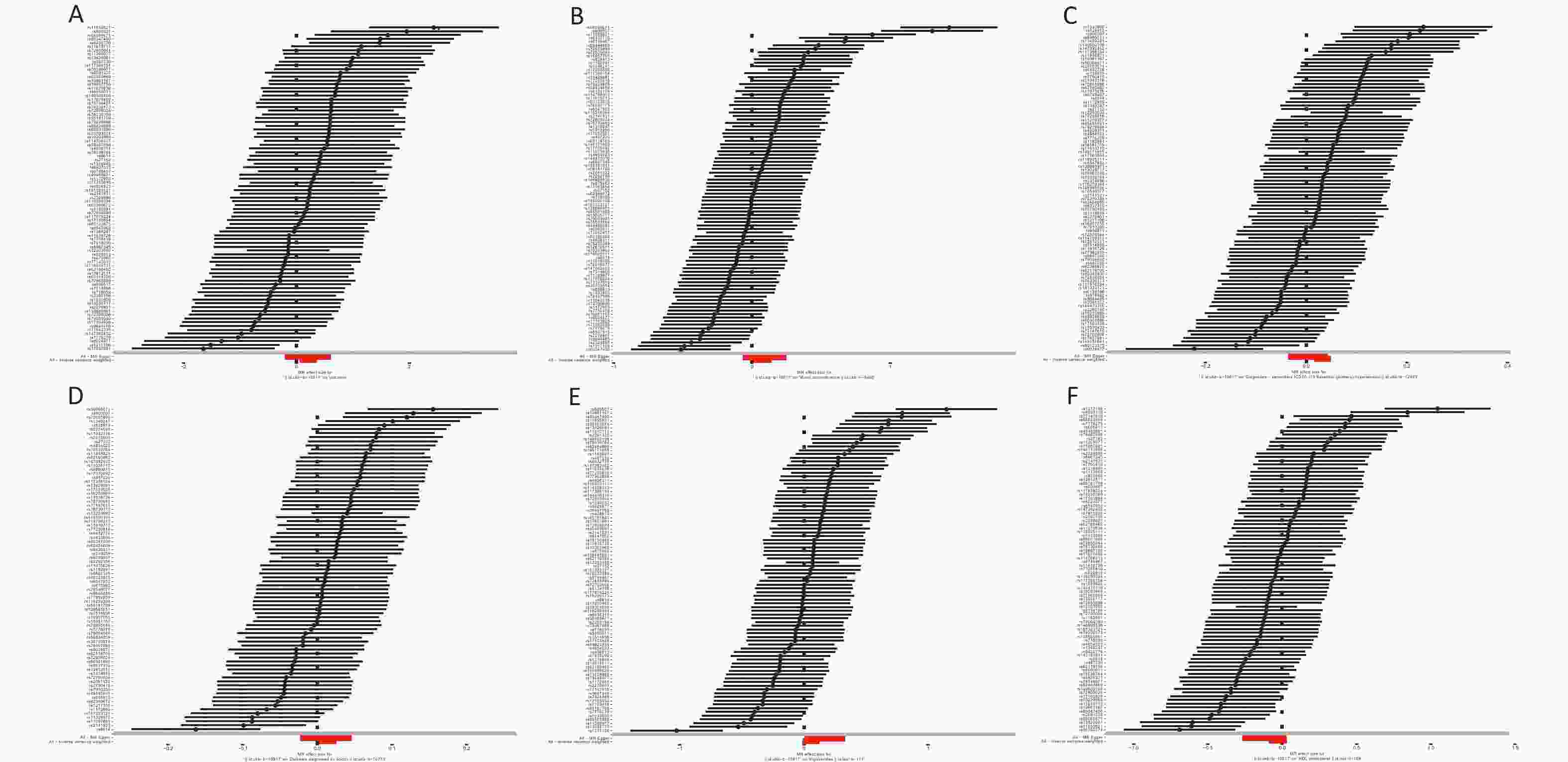
Figure S2. Forest plot of the association between PM2.5 and T2DM risk. (A) PM2.5 on MS. (B) PM2.5 on WA. (C) PM2.5 on HTN. (D) PM2.5 on DM. (E) PM2.5 on TG. (F) PM2.5 on HDL-C. X-axis shows the magnitude of the MR effect of PM2.5 on MS and its components, while the Y-axis shows the effect of each SNP.
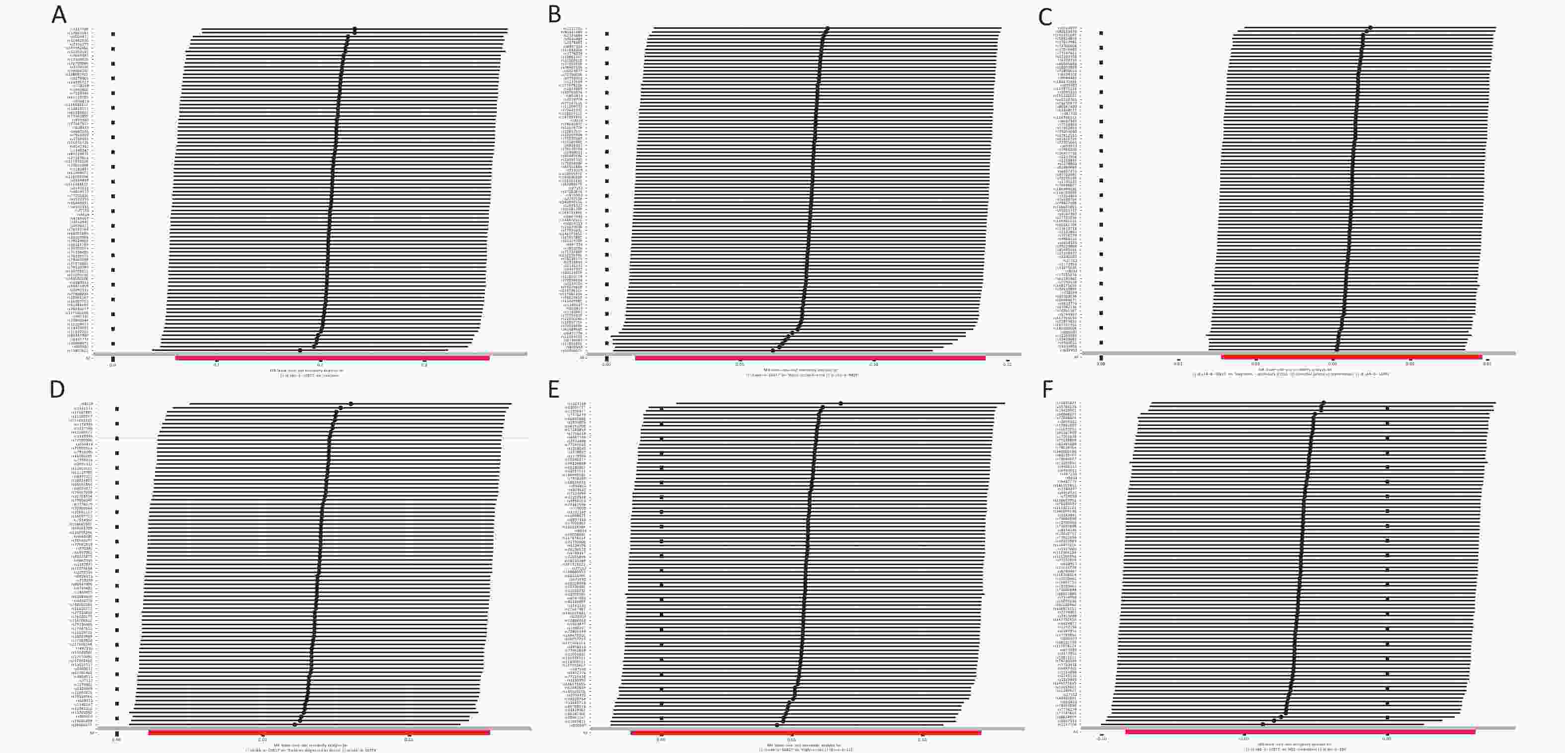
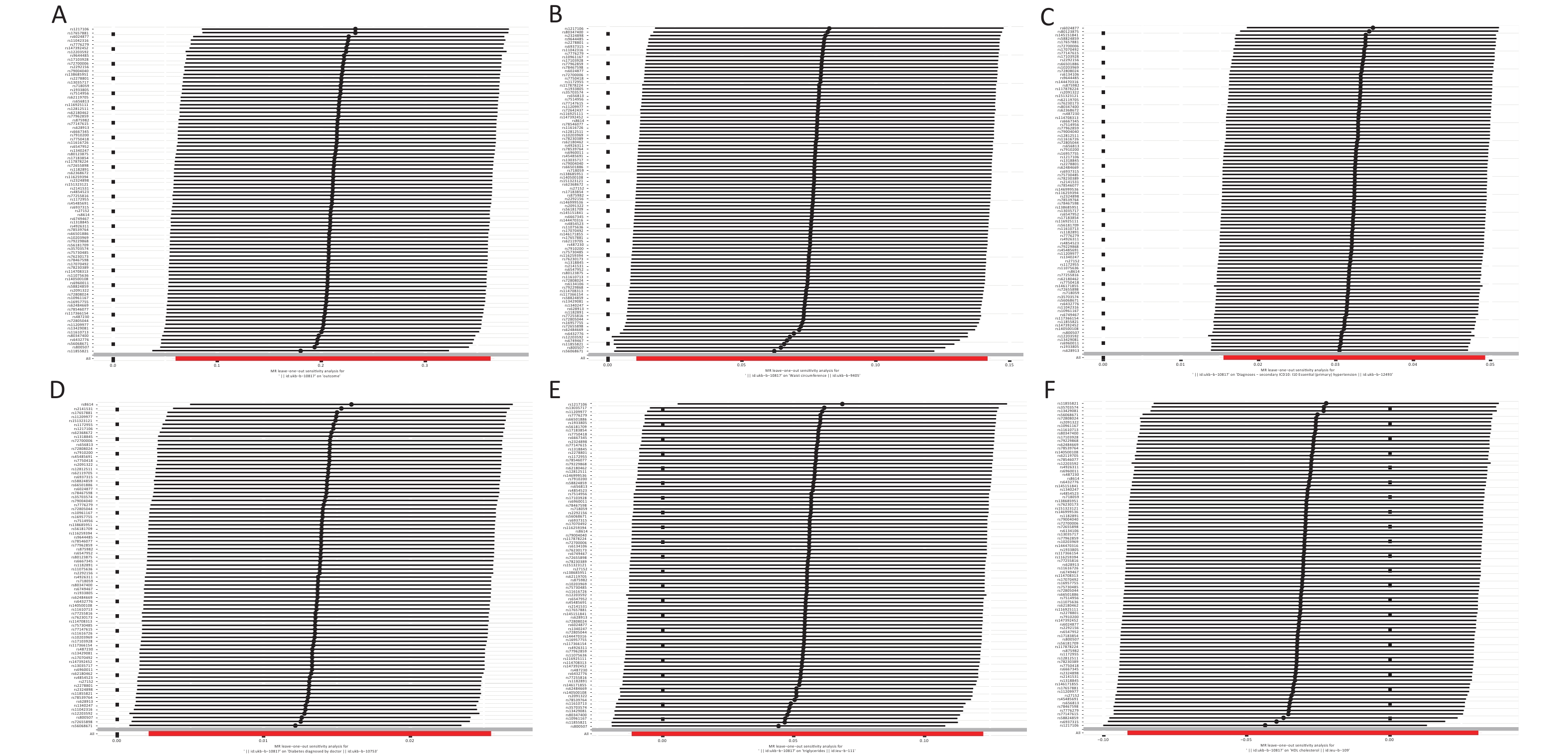
Figure S3. Results of sensitivity analysis using the leave-one-out method (A) PM2.5 on MS. (B) PM2.5 on WA. (C) PM2.5 on HTN. (D) PM2.5 on DM. (E) PM2.5 on TG. (F) PM2.5 on HDL-C.
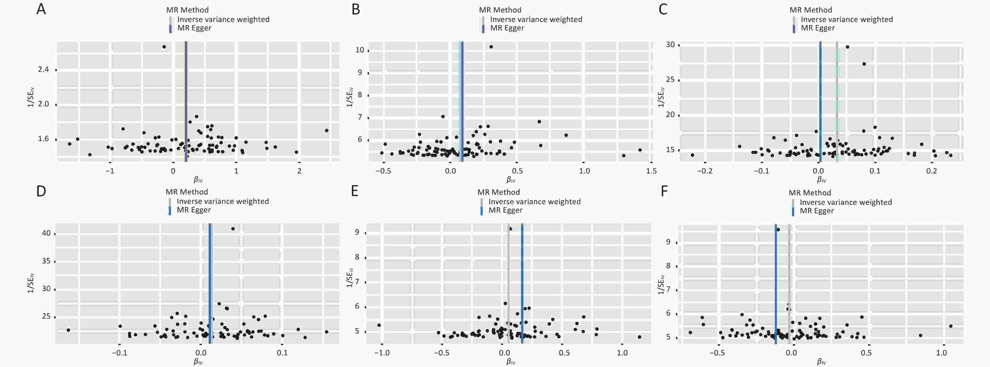
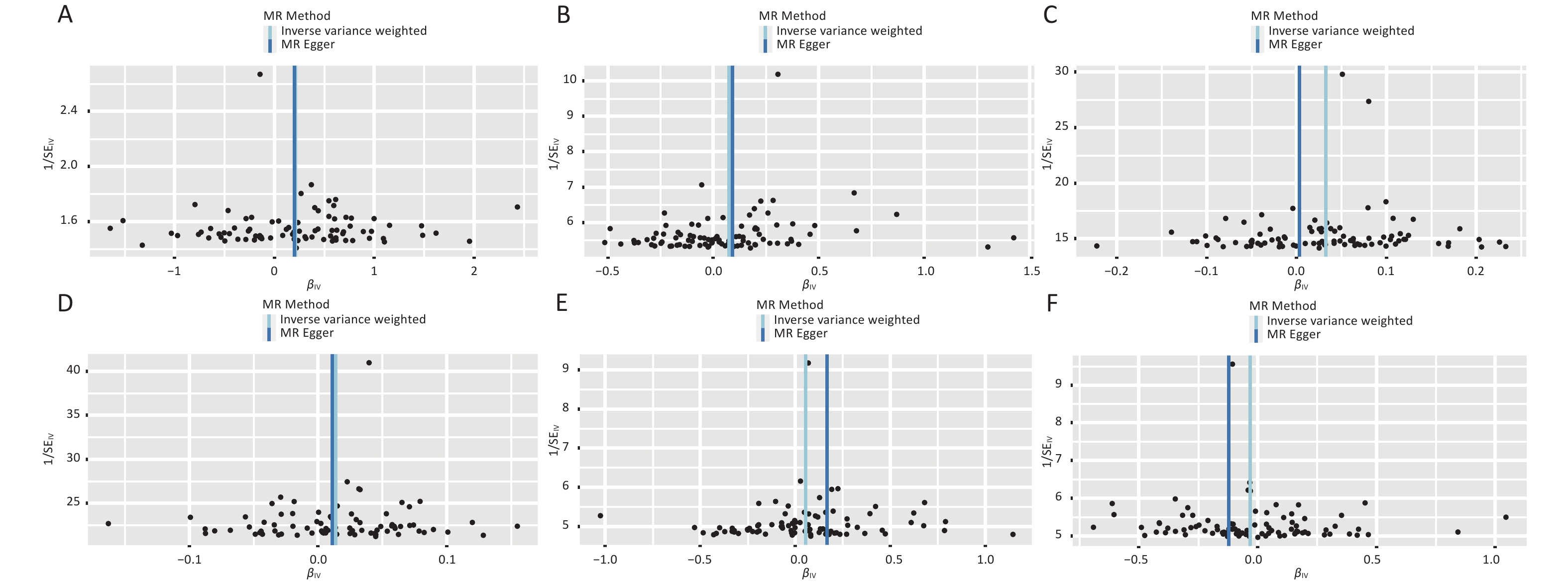
Figure S4. Funnel plot of PM2.5 on MS Mendelian randomization analysis (A) PM2.5 on MS. (B) PM2.5 on WA. (C) PM2.5 on HTN. (D) PM2.5 on DM. (E) PM2.5 on TG. (F) PM2.5 on HDL-C.
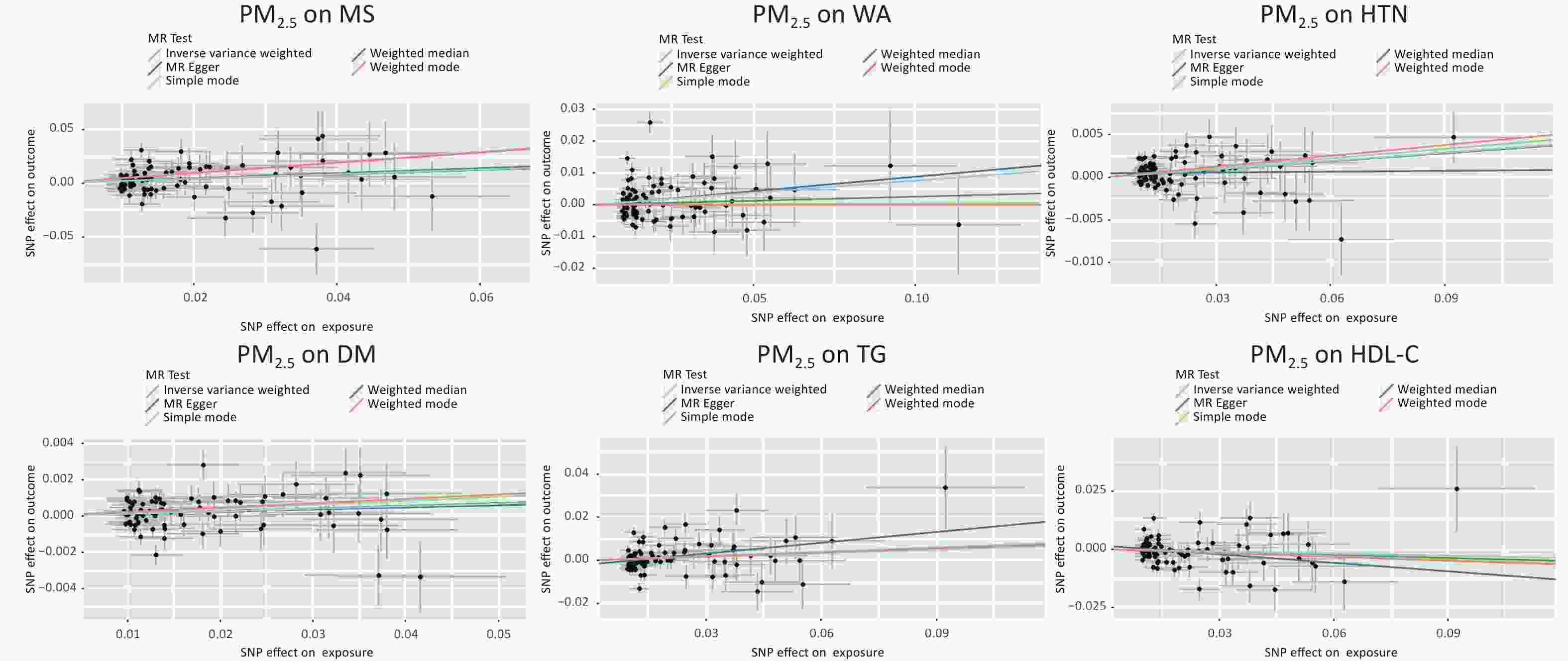
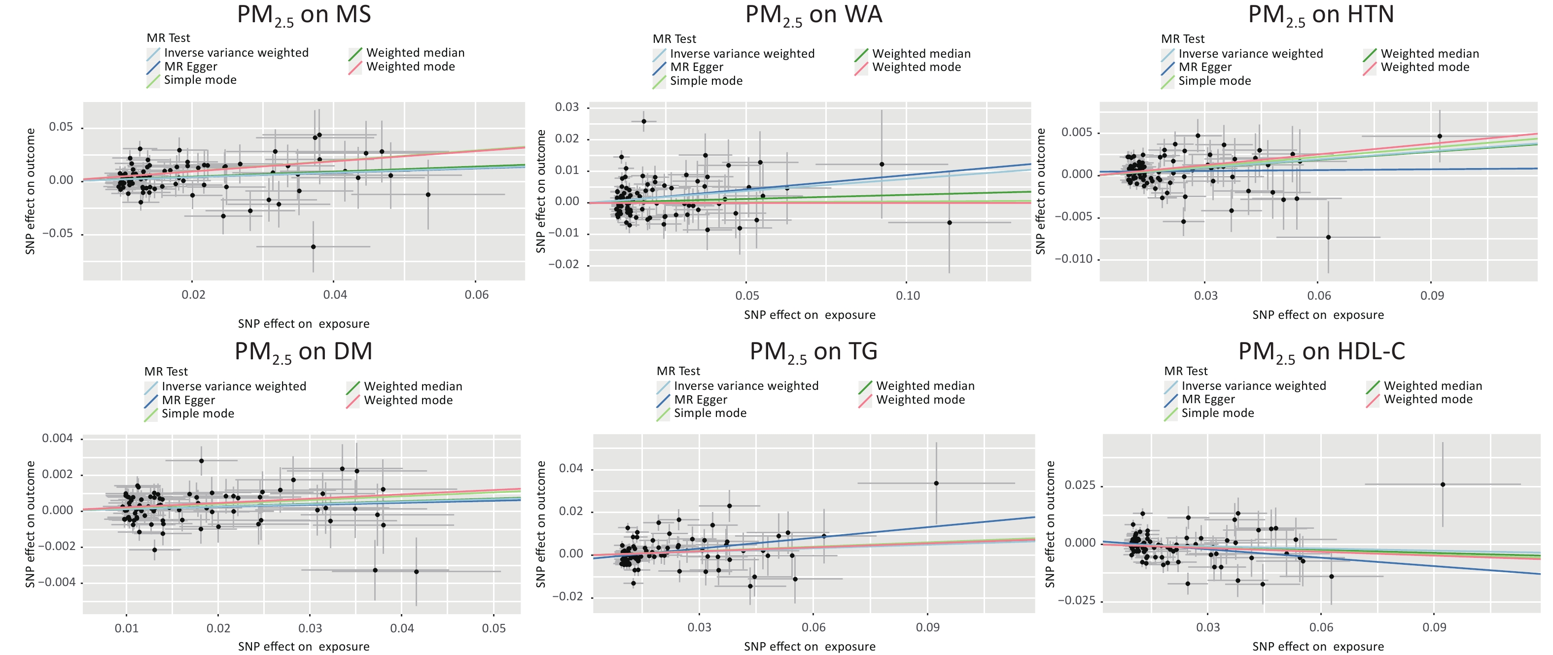
Figure S5. Individual SNP estimates of the causal effect of PM2.5 on MS and its components. The X-axis is the PM2.5 effect for each SNP, and the Y-axis is the effect of MS and components for each SNP. Regression lines for several methods are also given for MR-egger, weighted median, inverse variance weighted, simple mode and weighted mode.
全文HTML
 24202+.pdf
|

|

 Quick Links