

 下载:
下载:


-
The COVID-19 pandemic has wreaked havoc around the globe and caused significant disruptions across multiple domains[1]. Moreover, different countries have been differentially impacted by COVID-19 — a phenomenon that is due to a multitude of complex and often interacting determinants[2]. Understanding such complexity and interacting factors requires both compelling theory and appropriate data analytic techniques. Regarding data analysis, one question that arises is how to analyze extremely non-normal data, such as those variables evidencing L-shaped distributions. A second question concerns the appropriate selection of a predictive modelling technique when the predictors derive from multiple domains (e.g., testing-related variables, population density), and both main effects and interactions are examined.
To address these questions, we propose a novel statistical approach for analyzing and understanding complex data interactions. Using data collected in the USA during the first month in which COVID-19 testing was performed (March of 2020 Supplementary Table S1 available in www.besjournal.com), we examined the following six predictors of COVID-19 related deaths: (i) the proportion of all tests conducted during the first week of testing; (ii) the cumulative number of (test-positive) cases through 3-31-2020; (iii) the number of tests performed/million inhabitants; (iv) the cumulative number of inhabitants tested; (v) the number of cases/million inhabitants (cases/mill inh); and (vi) the number of diagnostic tests performed in week one of testing/million inhabitants/state-specific population density (w1DT/MI/PD), where “population density” is defined as the number of inhabitants per square kilometer.
Table S1. Epidemic data collected in all states of the USA in March, 2020
State Tests
wk ITotal
testsWk I/all
tests (%)State
pop/millTotal tests/
mill inhTotal
casesCases/
mill inhState
pop densWk I tests/
mill inh/state
pop densTotal deaths
(count)Deaths/
mill inhAK 227 3,654 6.21 0.734 4978.20 114 155.31 0.425 726.115 3 4.08 AL 352 5,014 7.02 4.908 1021.60 830 169.11 36.149 1.984 4 0.81 AR 115 3,453 3.33 3.038 1136.60 426 140.22 22.057 1.716 6 1.97 AZ 373 13,872 2.68 7.378 1880.18 919 124.56 24.990 2.023 17 2.30 CA 4,260 90,657 4.69 39.937 2270.00 5,708 142.93 94.198 1.132 123 3.07 CO 938 14,470 6.48 5.845 2475.62 2,307 394.70 21.680 7.402 47 8.04 CT 551 11,900 4.63 3.563 3339.88 1,993 559.36 248.188 0.623 34 9.54 DE 129 3,701 3.48 0.982 3768.84 236 240.33 152.342 0.862 6 6.11 FL 1,380 48,998 2.81 21.992 2227.99 4,950 225.08 129.126 0.485 59 2.68 GA 48 12,596 0.38 3.991 3156.10 2,683 672.26 25.930 0.463 80 20.04 HI 12 8,013 0.14 1.412 5674.93 175 123.93 49.869 0.170 0 0 ID 427 4,706 9.07 1.826 2577.22 310 169.77 8.436 27.718 6 3.28 IL 1,622 27,762 5.84 12.659 2193.06 4,596 363.06 84.395 1.518 66 5.21 IN 149 9,830 1.51 6.745 1457.38 1,514 224.46 71.505 0.308 32 4.74 IO 330 5,349 6.16 3.179 1682.60 336 105.69 21.811 4.759 4 1.25 KS 167 4,513 3.70 2.910 1550.86 319 109.62 13.655 4.202 6 2.06 KY 207 6,018 3.43 4.499 1337.63 439 97.57 42.988 1.070 9 2.00 LA 368 27,871 1.32 4.645 6000.22 3,540 762.11 34.240 2.313 151 32.50 MA 171 39,066 0.43 6.976 5600.06 4,955 710.29 255.203 0.096 48 6.88 MD 447 13,593 3.28 6.083 2234.59 1,239 203.68 189.312 0.388 10 1.64 ME 272 3,647 7.45 1.345 2711.52 253 188.10 14.677 13.777 3 2.23 MI 274 17,379 1.57 10.045 1730.11 5,486 546.14 40.101 0.680 132 13.14 MN 889 17,657 5.03 5.700 3097.72 503 88.24 25.314 6.161 9 1.57 MO 236 14,107 1.67 6.169 2286.76 903 146.37 34.169 1.119 12 1.94 MS 969 3,318 29.20 2.989 1110.07 758 253.59 23.828 13.605 14 4.68 MT 160 4,069 3.93 1.086 3746.78 161 148.25 2.851 51.664 1 0.92 NC 17 19,072 0.08 10.611 1797.38 1,167 109.98 76.123 0.021 5 0.47 ND 393 3724 10.55 0.761 4893.56 98 128.77 4.156 124.260 1 1.31 NE 272 2345 11.59 1.952 1201.33 120 61.47 8.859 15.728 2 1.02 NH 232 5,396 4.29 1.371 3935.81 258 188.18 56.622 2.988 3 2.18 NJ 284 35,602 0.79 8.936 3984.11 13,386 1497.99 395.555 0.080 161 18.01 NM 488 11,179 4.36 2.096 5333.49 237 113.07 5.944 39.168 2 0.95 NY 1,661 172,360 0.96 19.440 8866.26 59,513 3061.37 137.582 0.621 965 49.63 NV 262 10,534 2.48 3.139 3355.85 920 293.08 10.960 7.614 15 4.77 OH 148 20,665 0.71 11.747 1759.17 1,653 140.72 101.180 0.124 29 2.46 OK 206 1,634 12.60 3.954 413.25 429 108.50 21.840 2.385 16 4.04 OR 1,023 11,426 8.95 4.301 2656.59 548 127.41 16.879 14.090 13 3.02 PA 403 33,455 1.20 12.820 2609.59 3,394 264.74 107.478 0.292 38 2.96 RI 550 3,134 17.54 1.056 2967.80 294 278.40 263.934 1.973 3 2.84 SC 97 3,789 2.56 5.210 727.26 774 148.56 62.822 0.296 16 3.07 SD 185 3,218 5.74 0.903 3563.68 90 99.66 4.521 45.315 1 1.10 TN 73 20,574 0.35 6.897 2983.04 1,537 222.85 63.186 0.167 7 1.01 TX 48 25,760 0.18 29.472 874.05 2,552 86.59 42.365 0.038 34 1.15 UT 279 13,993 1.99 3.282 4263.56 719 219.07 14.926 5.695 2 0.60 VA 314 10,609 2.95 8.626 1229.89 890 103.17 77.861 0.467 22 2.55 VT 291 3701 7.86 0.628 5893.31 235 374.20 25.215 18.376 12 19.10 WA 4,415 59,206 7.45 7.797 7593.43 4,310 552.78 42.223 13.410 189 24.24 WI 259 17,662 1.46 5.851 3018.63 1,112 190.05 34.491 1.283 13 2.22 WV 38 3,108 1.22 1.778 1748.03 124 69.74 28.331 0.754 0 0 WY 308 1,641 18.76 0.567 2894.18 87 153.43 2.238 242.707 0 0 Note. Abbreviations of USA states: AK (Alaska), AL (Alabama), AR (Arkansas), AZ (Arizona), CA (California), CO (Colorado), CT (Connecticut), DE (Delaware), FL (Florida), GA (Georgia), HI (Hawaii), ID (Idaho), IL (Illinois), IN (Indiana), IO (Iowa), KS (Kansas), KY (Kentucky), LA (Louisiana), MA (Massachusetts), MD (Maryland), ME (Maine), MI (Michigan), MN (Minnesota), MO (Missouri), MS (Mississippi), MT (Montana), NC (North Carolina), ND (North Dakota), NE (Nebraska), NH (New Hampshire), NJ (New Jersey), NM (New Mexico), NY (New York), NV (Nevada), OH (Ohio), OK (Oklahoma), OR (Oregon), PA (Pennsylvania), RI (Rhode Island), SC (South Carolina), SD (South Dakota), TN (Tennessee), TX (Texas), UT (Utah), VA (Virginia), VT (Vermont), WA (Washington), WI (Wisconsin), WV (West Virginia), WY (Wyoming). Variables: Tests wk I = number of tests performed in the first 7 days of testing; Total tests = total number of people tested; Wk I/all tests (%) = tests wk I/total tests (i.e., the proportion of all tests conducted during the first week of testing, expressed as a percentage of all tests performed in March, 2020); State pop/mill = the population of each state, expressed in million inhabitants; Total tests/mill inh = number of tests performed per 1 million inhabitants by March 31, 2020; Total cases = cumulative number of confirmed (test-positive) infections by March 31, 2020; Cases/mill inh = the number of cases in the population (expressed in million inhabitants); State pop dens = the state-specific number of inhabitants per square kilometer; Wk I tests/mill inh/state pop dens = the number of tests performed during week one/million inhabitants/state population density; Total deaths (count) = cumulative number of deaths through March 31, 2020; Deaths/mill inh = cumulative number of deaths per 1 million inhabitants through March 31, 2020. The purpose of this study was to examine the ability of the six variables to predict COVID-19 related deaths in the United States during March of 2020. We ran the predictive model twice, once for each dependent variable: mortality count (overall number of deaths), and deaths per million inhabitants. Because our model (a) uses predictors that leverage information from multiple domains, (b) captures both nationwide and state-specific dimensions, and (c) examines two different mortality-related outcomes, the results are expected to have relevance for policy-makers.
All data used in this study were obtained from three sources in the public domain: Worldometer (
https://www.worldometers.info/coronavirus/ ), World Population Review (https://worldpopulationreview.com/states ), and Covidtracking(https://covidtracking.com/ ). The data were processed and analyzed using IBM SPSS, Minitab, and R. Univariate skewness and kurtosis values indicated that all predictors and outcomes were non-normally distributed, with a few variables evidencing L-shaped distributions. The L-shaped variables were normalized using the rank-based inverse normal (RIN) transformation[3]. For extremely non-normal data, the RIN method is a highly effective normalizing transformation[3].The prediction models were first examined using linear multiple regression, with the RIN-transformed versions of all variables used in the regressions. Because the homoscedasticity assumption (i.e., constant variance of the predicted Y-values) was not met, we re-ran the prediction models using a non-parametric approach known as Kernel Regularized Least Squares (KRLS) Regression[4]. KRLS is an appropriate method to use when the assumptions of linear regression are not met and the precise functional forms between the predictors and outcomes are unknown. All KRLS regressions used the RIN-transformed variables and all analyses were performed using the KRLS package for R. The use of non-parametric, machine learning-based methods such as KRLS is consistent with recent calls to place greater reliance on artificial intelligence systems for understanding the causes and consequences of the COVID-19 pandemic[5].
The KRLS regression results are presented in Table 1. For number of deaths, the six predictors accounted for 98.8% of the variance. Five of the predictors were statistically significant (P-values ≤ 0.002). Two of the significant predictors (i.e., number of test-positive cases, Cohen’s d = 2.3; and cases per million inhabitants, Cohen’s d = 1.3) represent different ways of quantifying the illness burden due to SARS-CoV-2 infection. The ratio of the two d values indicated that the predictive strength of number of test-positive cases was 77% greater than was cases per million inhabitants. Regarding the second dependent variable, the six predictors accounted for 92.6% of the variance in deaths per million inhabitants. Five of the predictors were significant (P-values ≤ 0.03). For this regression analysis, the number of test-positive cases (d = 1.1) and cases per million inhabitants (d = 1.4) were similar in predictive strength.
Table 1. KRLS regression of potential predictors of COVID-19 related mortality
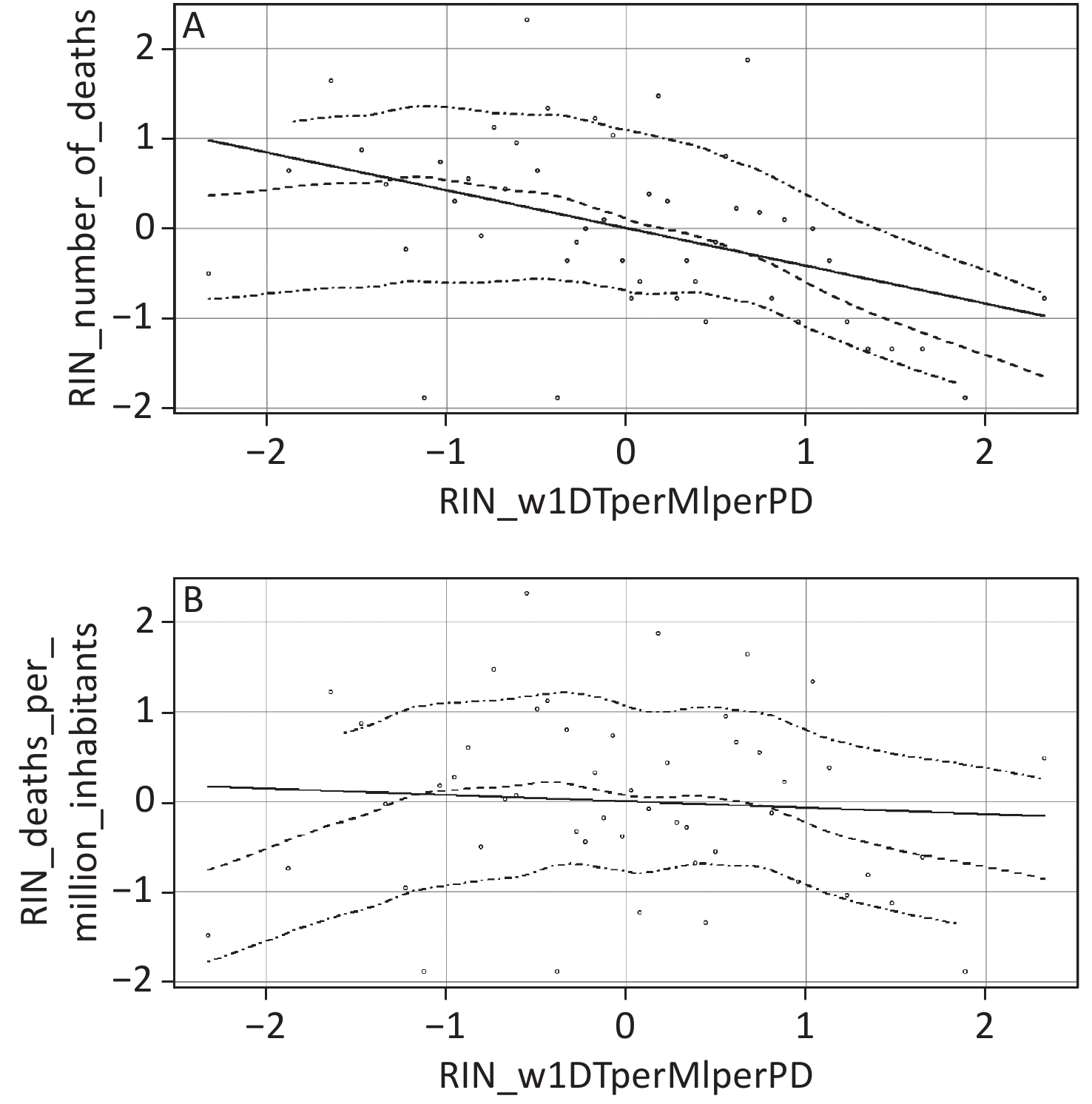
Items Estimate Std. Error t value P-value Predictors of number of deaths Totaltests RIN 0.111 0.033 3.326 0.002 Testedpermil RIN −0.153 0.026 −5.782 < 0.001 Wkonepropalltests RIN 0.044 0.030 1.452 0.153 Wkonepermilcitperpopden RIN 0.169 0.032 5.262 < 0.001 Confircases RIN 0.568 0.035 16.340 < 0.001 Casespermil RIN 0.215 0.023 9.185 < 0.001 Predictors of deaths per million inhabitants Totaltests RIN −0.138 0.058 −2.352 0.023 Testedpermil RIN 0.004 0.048 0.091 0.928 Wkonepropalltests RIN 0.136 0.061 2.234 0.031 Wkonepermilcitperpopden RIN 0.161 0.063 2.570 0.014 Confircases RIN 0.408 0.055 7.353 < 0.001 Casespermil RIN 0.441 0.045 9.748 < 0.001 Note. All predictors were normalized using the rank-based inverse normal (RIN) transformation. Estimates are sample-average partial derivatives. The set of predictors accounted for 98.8% of the variance in number of deaths (R2 = 0.9875). For deaths per million citizens, the predictors accounted for 92.6% of the variance (R2 = 0.9264). Description of predictors: totaltests = number of tests performed in March of 2020; testedpermil = number of all tests conducted per million inhabitants, in March of 2020; wkonepropalltests = all tests conducted during the first week of testing, expressed as the percentage of all tests performed in March 2020; wkonepermilcitperpopden = the number of tests performed during week one per million inhabitants, divided by state-specific population density; confircases = total number of test-positive individuals, in March of 2020; casespermil = number of test-positive individuals per million inhabitants, in March of 2020. In addition to number of test-positive cases and cases per million inhabitants, another interesting predictor was our geo-demographic variable (i.e., the number of diagnostic tests/million inhabitants/population density performed in week one of testing, or w1DT/MI/PD). This predictor was significantly associated with both dependent variables. Because w1DT/MI/PD is a complex, ratio-based predictor, discerning the precise nature of its predictive association from a single regression estimate alone is challenging. To further enhance the interpretation of this variable, we created two scatterplots showing the association between w1DT/MI/PD and each dependent variable. Both scatterplots include a best fitting linear regression line and a lowess line (with accompanying 95% confidence interval). Lowess stands for locally weighted scatterplot smoothing. The lowess line is the best fitting non-linear curve that tracks the data points in the scatterplot. The lowess curves allow us to make inferences about COVID-19 related deaths at low and high levels of w1DT/MI/PD. Such inferences are tantamount to examining COVID-19 related deaths for U.S. states scoring low versus high on the geo-demographic predictor variable. The scatterplots were created using the car package for R.
As the lowess curve in the top panel of Figure 1 indicates, at higher and medium levels of w1DT/MI/PD, the association between the geo-demographic predictor and death count was strongly negative and moderately negative, respectively. In contrast, at lower levels of w1DT/MI/PD, there was little if any association between the geo-demographic variable and number of fatalities. The bottom panel of Figure 1 indicates that at lower levels of w1DT/MI/PD, the association between the geo-demographic variable and deaths per million inhabitants was moderately positive. At medium levels of w1DT/MI/PD, there was little if any association between the two variables. Finally, at higher levels of w1DT/MI/PD, there was a moderately strong negative association between the geo-demographic variable and deaths per million inhabitants.
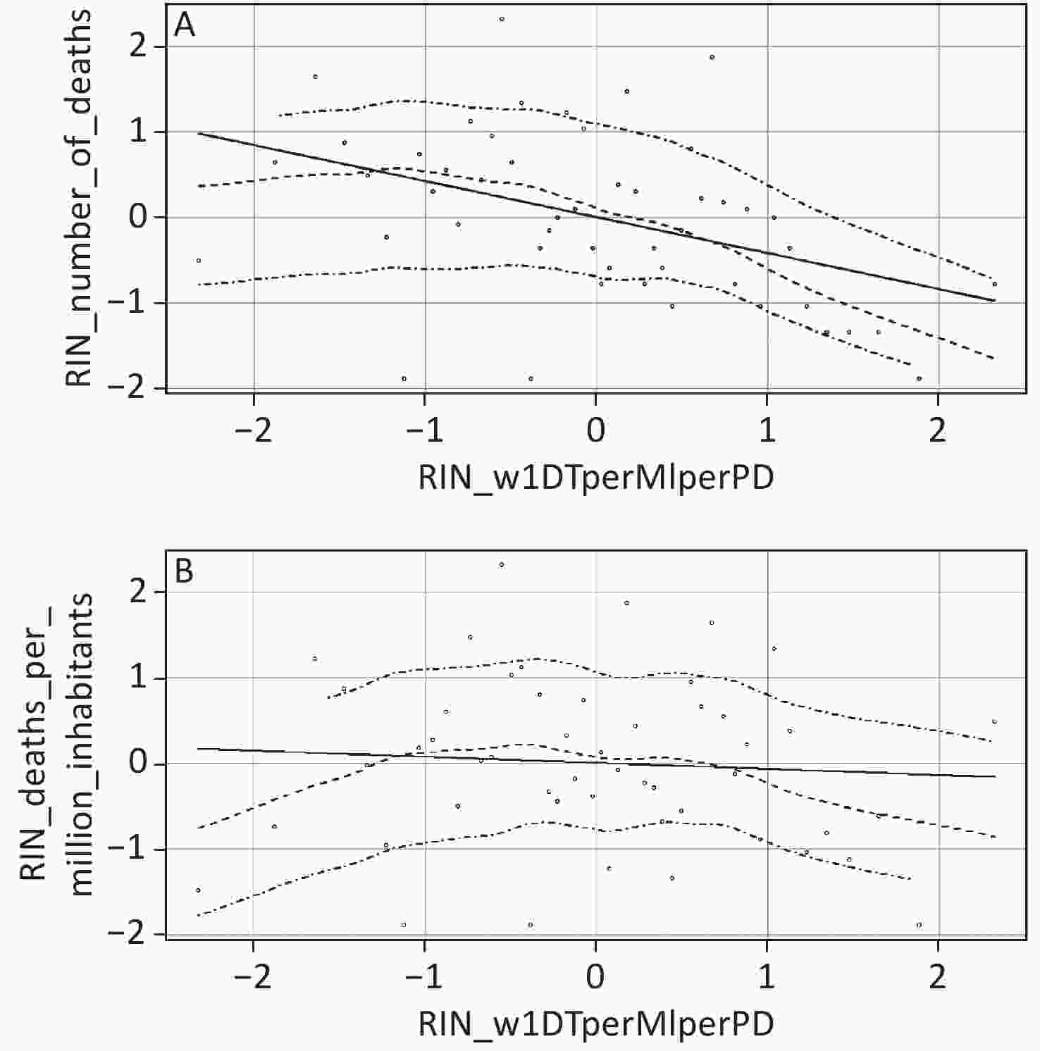
Figure 1. Scatterplots depicting lowess curves (the middle dashed lines) and accompanying 95% confidence intervals (top and bottom dashed lines) for the association between number of tests during week 1/million inhabitants/population density and (A) number of COVID-19 related deaths (top panel) and (B) number of COVID-19 related deaths per million inhabitants (bottom panel). All variables were normalized using the rank-based inverse normal (RIN) transformation.
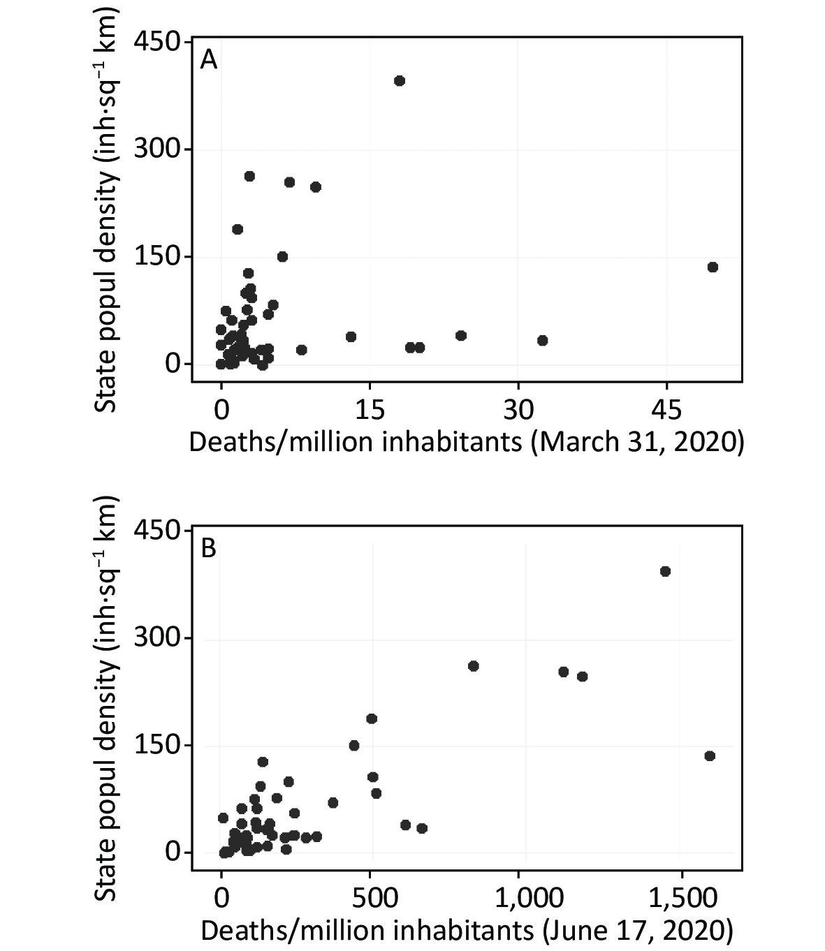
In constructing our geo-demographic predictor variable, we controlled for population density because it is an important factor associated with disease transmission[6]. Moreover, because there typically is a lag time of several weeks or more between being infected with SARS-CoV-2 and showing disease-related symptoms, the association between population density and disease-related deaths should strengthen over time. To highlight this point, Figure 2 presents scatterplots showing the Pearson correlations between population density and cumulative COVID-19 related deaths per million inhabitants through March 31st and June 17th, 2020, respectively. The correlations were as follow: March 31st (r = 0.228, P > 0.05); June 17th (r = 0.800, P < 0.01). The difference between the two statistically dependent correlations was evaluated using Hittner, May and Silver’s modification of Dunn and Clark’s z test[7]. The two correlations were significantly different (z = 5.85, P < 0.0001), thereby supporting the prediction that the association between population density and COVID-19 related deaths will strengthen over time.
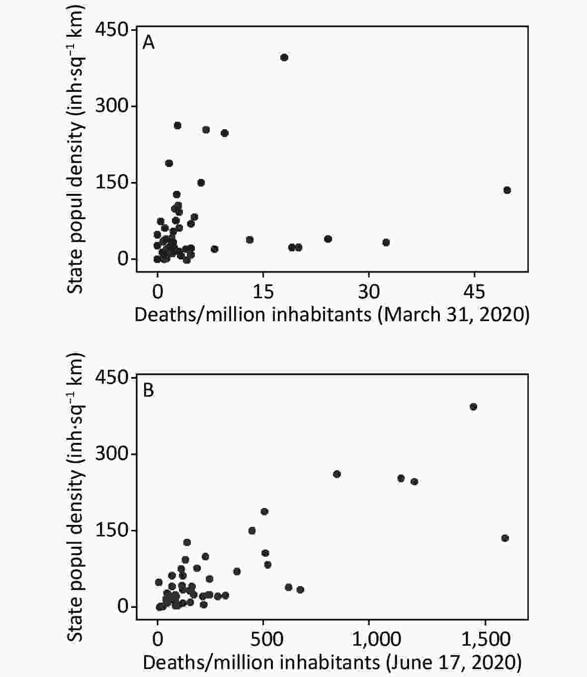
Figure 2. Scatterplots showing the Pearson correlations between population density and cumulative COVID-19 related deaths per million inhabitants through (A) March 31, 2020, top panel (r = 0.228, 95% CI: −0.054, 0.476) and (B) June 17, 2020, bottom panel (r = 0.80, 95% CI: 0.671, 0.882).
To the best of our knowledge, this is the first study that examines testing-, case count- and geo-demographic variables as predictors of COVID-19 related deaths. Using a flexible, machine learning-based approach (KRLS regression), we found that our predictors accounted for very high percentages of outcome variance (98.8% and 92.6% for number of deaths and deaths per million inhabitants, respectively). Furthermore, with very few exceptions, our predictors were both statistically significant and practically important.
One novel contribution of this study was our examination of a complex, ratio-based geo-demographic predictor variable. This variable—the number of diagnostic tests performed in week one of testing/million inhabitants/state-specific population density (w1DT/MI/PD)—significantly predicted COVID-19 related deaths, but did so differently depending on where, along the continuum of geo-demographic values, the predictive association was examined. At the lower end of the geo-demographic predictor, more tests during week one per million inhabitants, normalized by population density, were associated with more deaths per million citizens. In contrast, at the higher end of the geo-demographic predictor, more tests during week one per million inhabitants, normalized by population density, were associated with fewer deaths per million inhabitants. These different quantitative patterns could reflect different qualitative situations. In the first case (lower values on the geo-demographic variable, where more tests are associated with more deaths), testing seems to pursue a confirmatory purpose. In contrast, for the second case (higher values on the geo-demographic variable, where more tests are associated with fewer deaths), diagnostic testing appears to be emphasized[8]. One implication of these findings is that when examining our geo-demographic variable as a predictor of deaths, the inflection points along the lowess curves (the positions where the slope rises and falls) can serve as approximate cut-points demarcating three types of testing: confirmatory, diagnostic, and other.
When testing prioritizes symptomatic cases, it is expected that most tested individuals will result in positive results (infection will be confirmed). Because deaths will occur within a subset of infected individuals, when testing is confirmatory (when only symptomatic patients are tested), more tests will be associated with more deaths. In contrast, when asymptomatic individuals are also tested, more tests, conducted earlier, will allow clinicians to detect, treat, and isolate infections earlier and prevent further viral dissemination which, in turn, will result in fewer deaths/million inhabitants. Our findings thus support an important recommendation from the World Health Organization, which is that early and frequent testing helps to prevent deaths[9].
In addition to the contributions described above, we performed supplemental analyses examining the association between population density and COVID-19 related deaths. The role of population density in predicting epidemic dispersal and epidemic-related deaths is receiving increased research attention[10]. To the best of our knowledge, the present study is the first to demonstrate that the magnitude of association between population density and COVID-19 related deaths strengthens as the time since first infection increases. Understanding how factors such as testing frequency, the relative proportion of confirmatory versus diagnostic testing, and sociodemographic composition influence the temporal association between population density and COVID-19 related deaths is an important priority for future research.
Overall, our findings highlight the importance of considering predictor variables from multiple domains. When ratio-based predictors such as our geo-demographic variable are analyzed, we recommend examining lowess curves as a visual interpretational aid for explicating the (often) complex non-linear associations between such ratio-based predictors and various outcomes of interest. An important direction for future research on epidemic dissemination and potential control is to examine both ratio-based composite variables—such as our geo-demographic measure—and traditional multiplicative interaction terms (created as linear products of two or more variables). The joint examination of both types of complex variables might result in greater predictive power and/or might foster additional insights into the dynamics of infectious diseases, such as COVID-19.
This work was previously released as a preprint by J. B. Hittner, F. O. Fasina, A. L. Hoogesteijn, R. Piccinini, P. Kempaiah, S. D. Smith, and A. L. Rivas, with the title ‘Early and massive testing saves lives: COVID-19 related infections and deaths in the United States during March of 2020’ medRxiv 2020.05.14.20102483;
https://doi.org/10.1101/2020.05.14.20102483 .Acknowledgements The authors appreciate the data gathering efforts of those citizens who contributed to COVID-19 tracking (
https://covidtracking.com ). FOF is currently funded by the United States Agency for International Development (USAID) grant to the Food and Agriculture Organization of the United Nations, (Global Health Security Agenda- Zoonotic Diseases and Animal Health in Africa). The views and opinions expressed in this paper are those of the authors and not necessarily the views and opinions of the United States Agency for International Development and the Food and Agriculture Organization of the United Nations.Financial
Support This research received no specific grant from any funding agency, commercial or not-for-profit entity. Conflict of Interest The authors declare that they have no conflict of interest.
Author
Contributions JBH and ALR designed the study. DM curated the original data. ALH, RP, PK, SDS, JBH, and FOF reviewed the literature and extracted and filtered the available data from online repositories. JBH conducted the statistical analyses. All authors contributed to writing of the report.
全文HTML
 20319.pdf
|

|

 Quick Links